3  The waveform

3.1 Managing channels

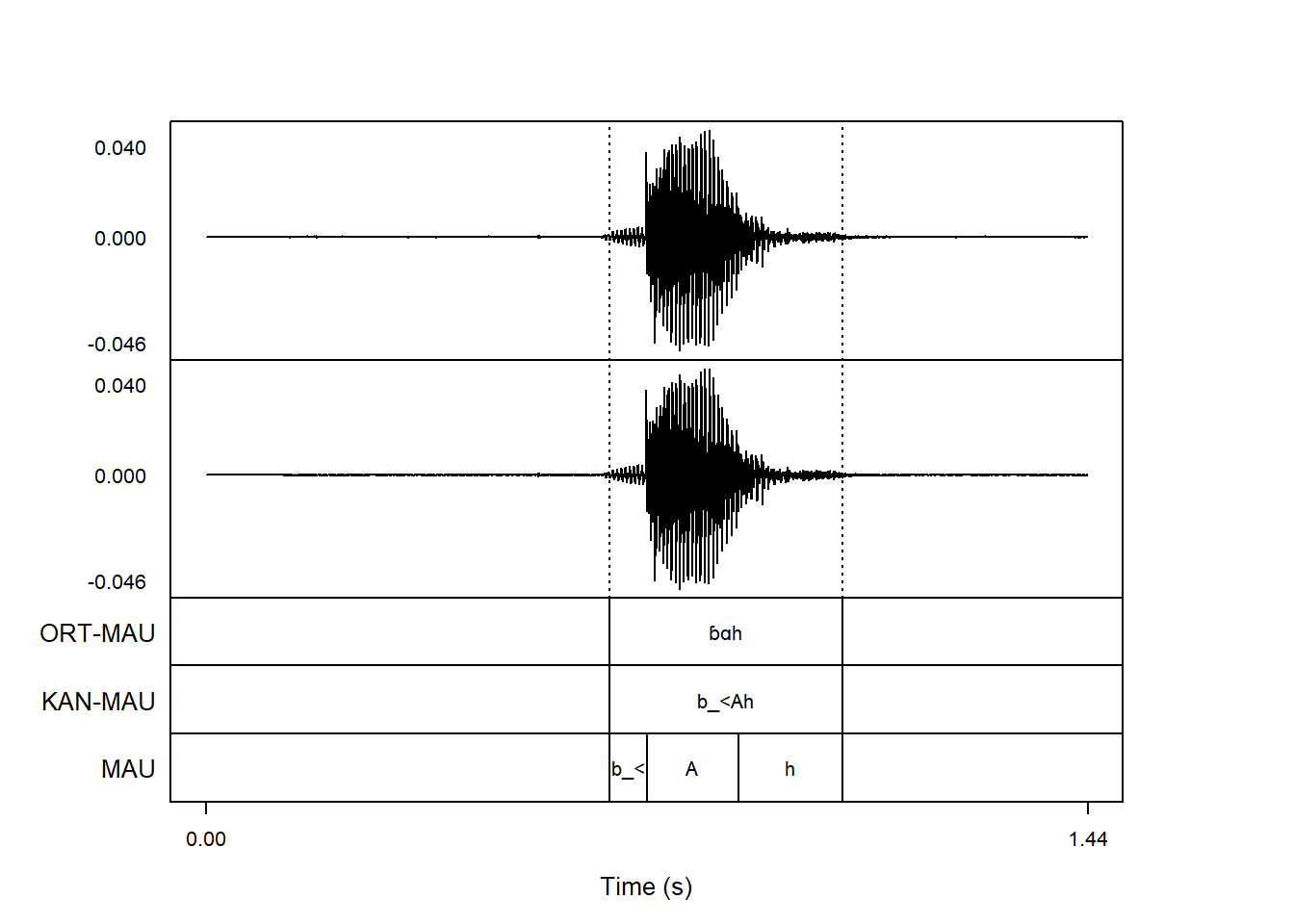
praatpicture() has the option of plotting multiple channels. By default, all channels are plotted. If you have a stereo sound file, it will look like this:

praatpicture('ex/index_stereo.wav', 
             frames = c('sound', 'TextGrid'),
             proportion = c(70, 30))

You may not want this; if you prefer plotting just a single channel, you can controls this with the wave_channels argument. For plotting just the second channel:

praatpicture('ex/index_stereo.wav', 
             frames = c('sound', 'TextGrid'),
             proportion = c(70, 30),
             wave_channels = 2)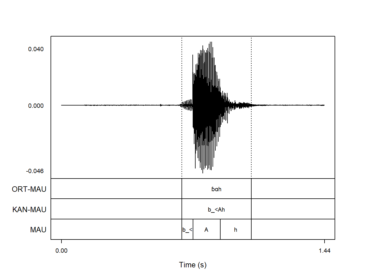

As indicated above, it is also possible plot audio with more than two channels, like in this case, where one channel captures audio, and other channels capture various articulatory signals:

praatpicture('ex/multichannel.wav', 
             start = 0.6, end = 2.4,
             frames = c('sound', 'TextGrid'),
             proportion = c(70, 30))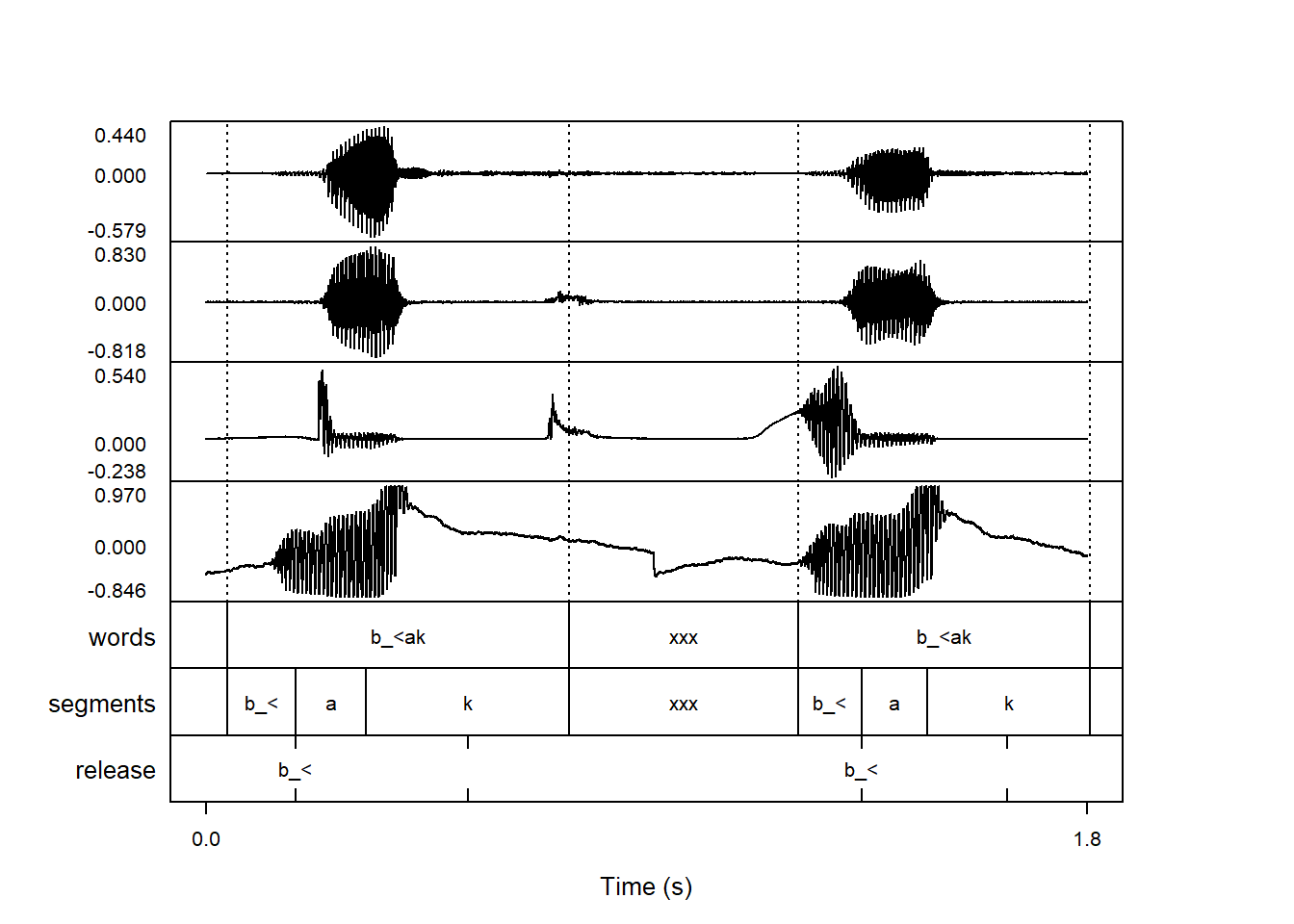

The argument wave_channels can be used to both extract and reorder channels. Here we omit the second channel, and swap the order of the third and fourth channels:

praatpicture('ex/multichannel.wav', 
             start = 0.6, end = 2.4,
             frames = c('sound', 'TextGrid'),
             proportion = c(70, 30),
             wave_channels = c(1,4,3))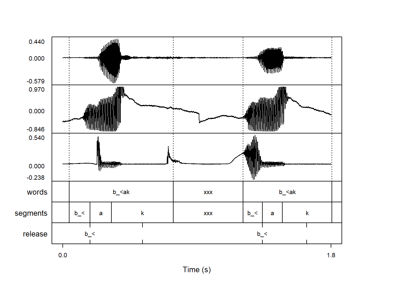

3.2 Labelling channels

The argument wave_channelNames can be used to add labels next to the y-axis with channel names. It is set to FALSE by default. If we plot stereo data with wave_channelNames set to TRUE, it’ll by default print the labels “left” and “right” next to the channels:

praatpicture('ex/index_stereo.wav', 
             frames = c('sound', 'TextGrid'),
             proportion = c(70, 30),
             wave_channelNames = TRUE)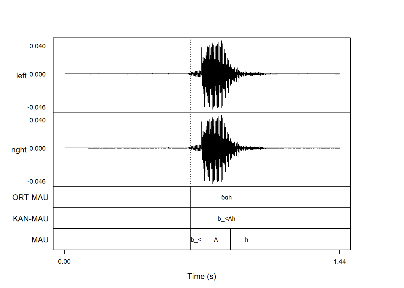

Instead of passing a logical argument like TRUE, we can also pass a vector of strings and thus control the channel labels:

praatpicture('ex/index_stereo.wav', 
             frames = c('sound', 'TextGrid'),
             proportion = c(70, 30),
             wave_channelNames = c('above', 'below'))

This is especially useful in cases like our multichannel data above, where we can then label the sources of the signals:

praatpicture('ex/multichannel.wav', 
             start = 0.6, end = 2.4,
             frames = c('sound', 'TextGrid'),
             proportion = c(70, 30),
             wave_channelNames = c('audio', 'airflow', 'EGG', 'Pio'))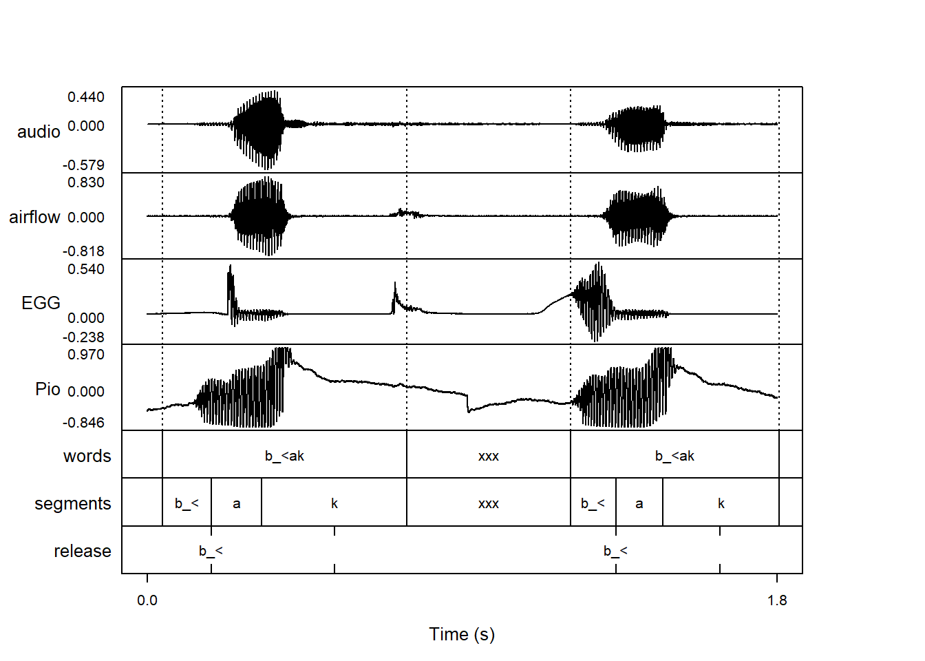

You can of course also label just a single channel:

praatpicture('ex/index.wav', 
             frames = c('sound', 'TextGrid'),
             proportion = c(70, 30),
             wave_channelNames = 'wave')

3.3 Coloring options

The argument wave_color allows users to control the color of the waveform. By default it is set to black; when plotting waveforms along with spectrogram, it is often the spectrogram in focus, so it can make a lot of sense to give the waveform a lighter grey color like so:

praatpicture('ex/index.wav', 
             wave_color='grey')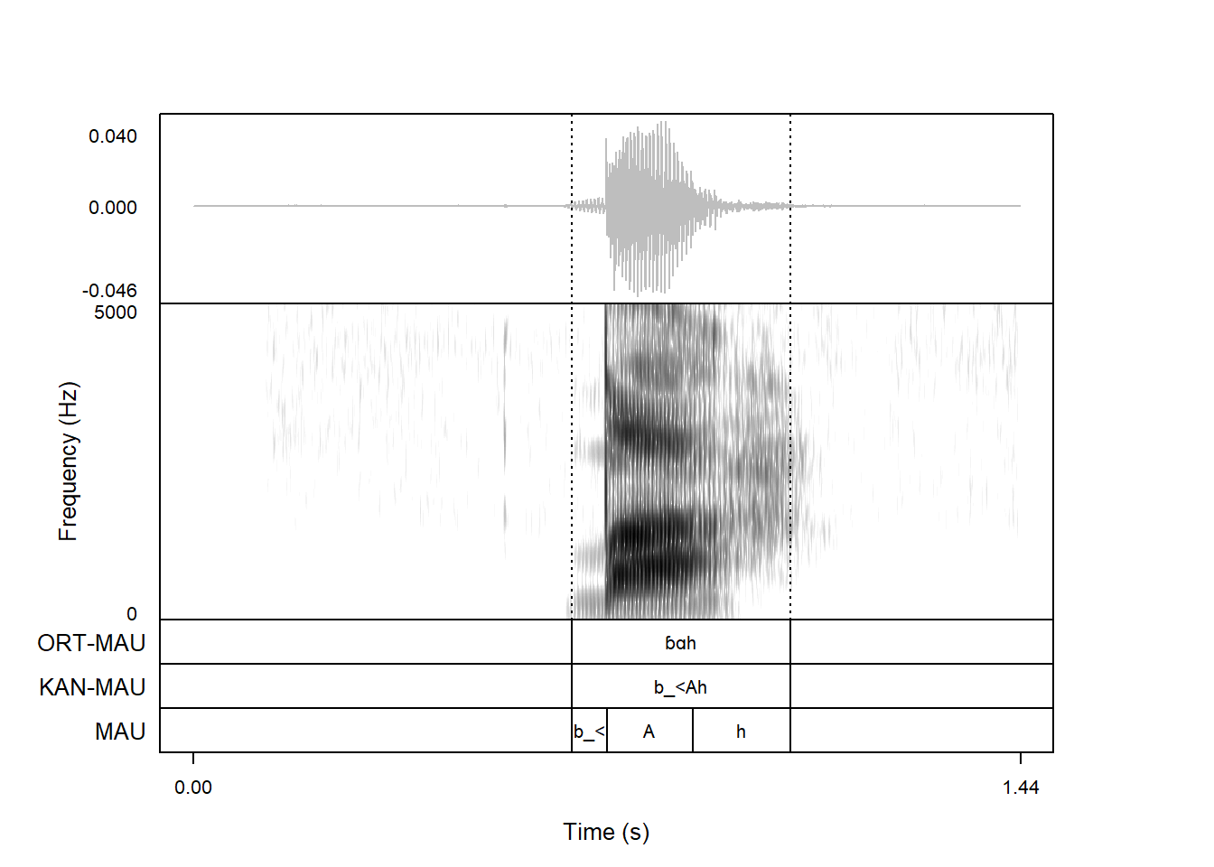

When multichannel data are plotted, it is also possible to assign different colors to different channels, by passing a vector instead of a single string to wave_color.

praatpicture('ex/multichannel.wav', 
             start = 0.6, end = 2.4,
             frames = c('sound', 'TextGrid'),
             proportion = c(70, 30),
             wave_channelNames = c('audio', 'airflow', 'Pio', 'EGG'),
             wave_color=c('red', 'black', 'orange', 'blue'))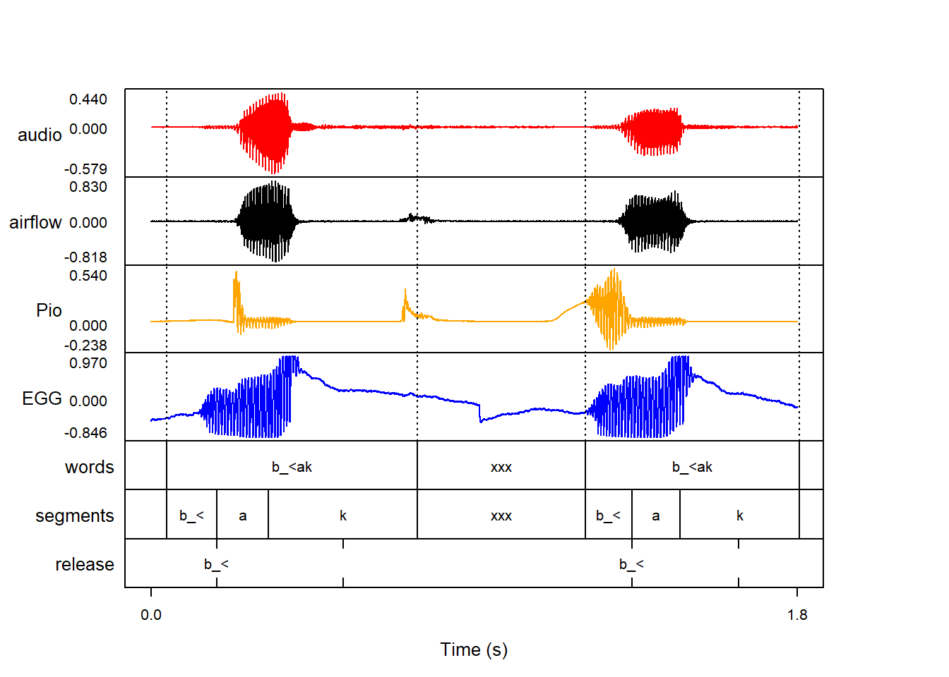

3.4 Line width

The width of the waveform line can be controlled with the wave_lineWidth argument. If you’re plotting a very complex wave, it can be helpful to pass a number smaller than 1, which is the default:

praatpicture('ex/index.wav', 
             frames = c('sound', 'TextGrid'),
             proportion = c(70, 30),
             wave_lineWidth = 0.5)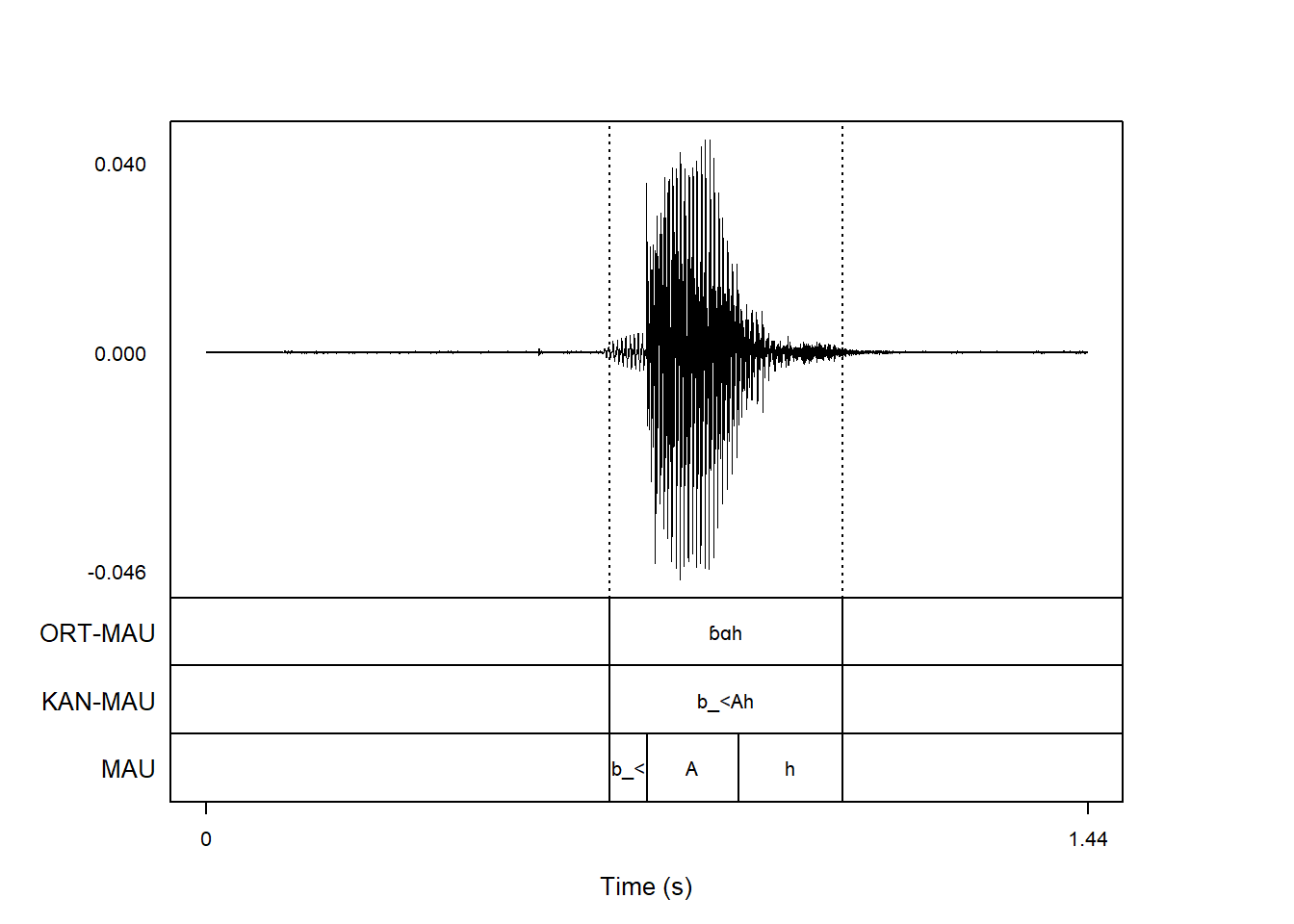

You typically won’t want to pass a number larger than 1, but it could make sense if you’re plotting only a very short sound snippet.

3.5 Appearance of the y-axis

The number of digits to be printed along the y-axis can be controlled with the wave_axisDigits argument. By default, 3 digits are shown, but it’s easy to print more if you want:

praatpicture('ex/index.wav', 
             frames = c('sound', 'TextGrid'),
             proportion = c(70, 30),
             wave_axisDigits = 5)

Often, these exact values don’t tell us all that much. You can suppress the y-axis entirely by setting wave_axisDigits = 0:

praatpicture('ex/index.wav', 
             frames = c('sound', 'TextGrid'),
             proportion = c(70, 30),
             wave_axisDigits = 0)