11 Annotating interactively in R

praatpicture is not designed to annotate sound files, something that Praat already does very well. But if you want to quickly make some simple annotations of a sound file and would for whatever reason prefer not to go through the process of making these in Praat, saving them in the right format, etc., there are simple functions available in praatpicture that allows you to do this interactively without leaving R. This is accomplished with the make_TextGrid() function.

11.1 Basic usage

The make_TextGrid function takes two obligatory arguments:

sound the name of a sound file to annotate
tierNames the names of desired annotation tiers

If we run the following code, two things should happen: for RStudio users, a playable sound file should up in the Viewer pane, and a graphics device window should open.

new_tg <- make_TextGrid('ex/index.wav',
                        tierNames = c('Mary', 'John', 'bell'))

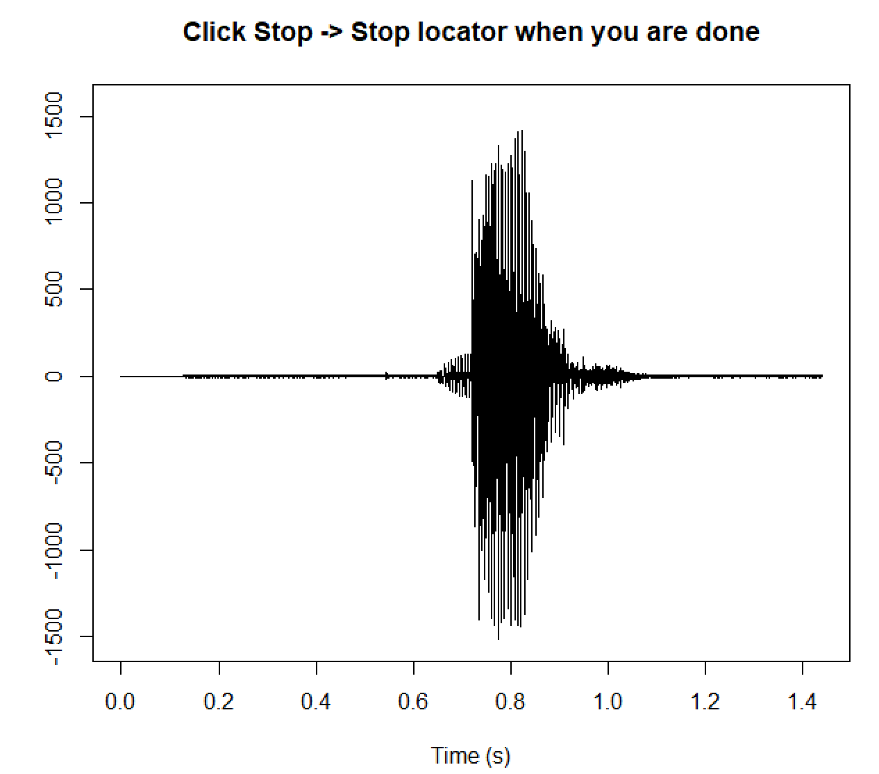
In the R console, you will see the following text:

Navigate to the graphics device window and click in the positions where you want TextGrid boundaries for tier Mary

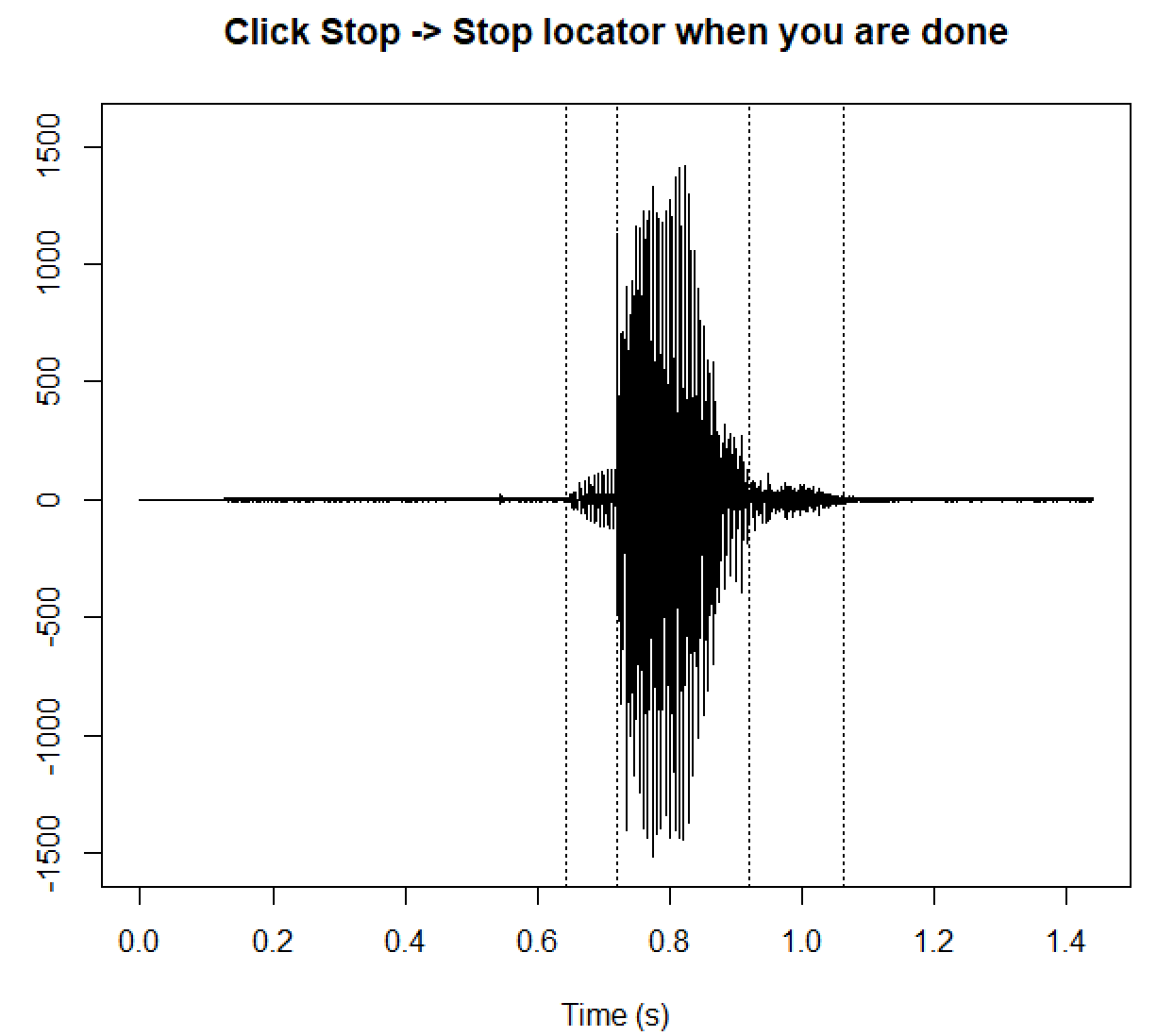
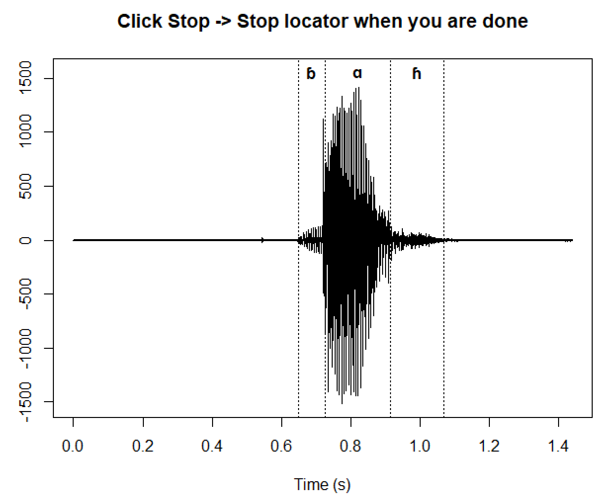
You can now click on the image where you want annotation boundaries to be. If you click the Stop locator button in the graphics window, you will see dotted lines in the locations where you clicked:

In the console, you will be asked the following question:

Is this an interval tier? [y/n]

I indeed had an interval tier, so I will type y and press enter! If you want a point tier, type n.

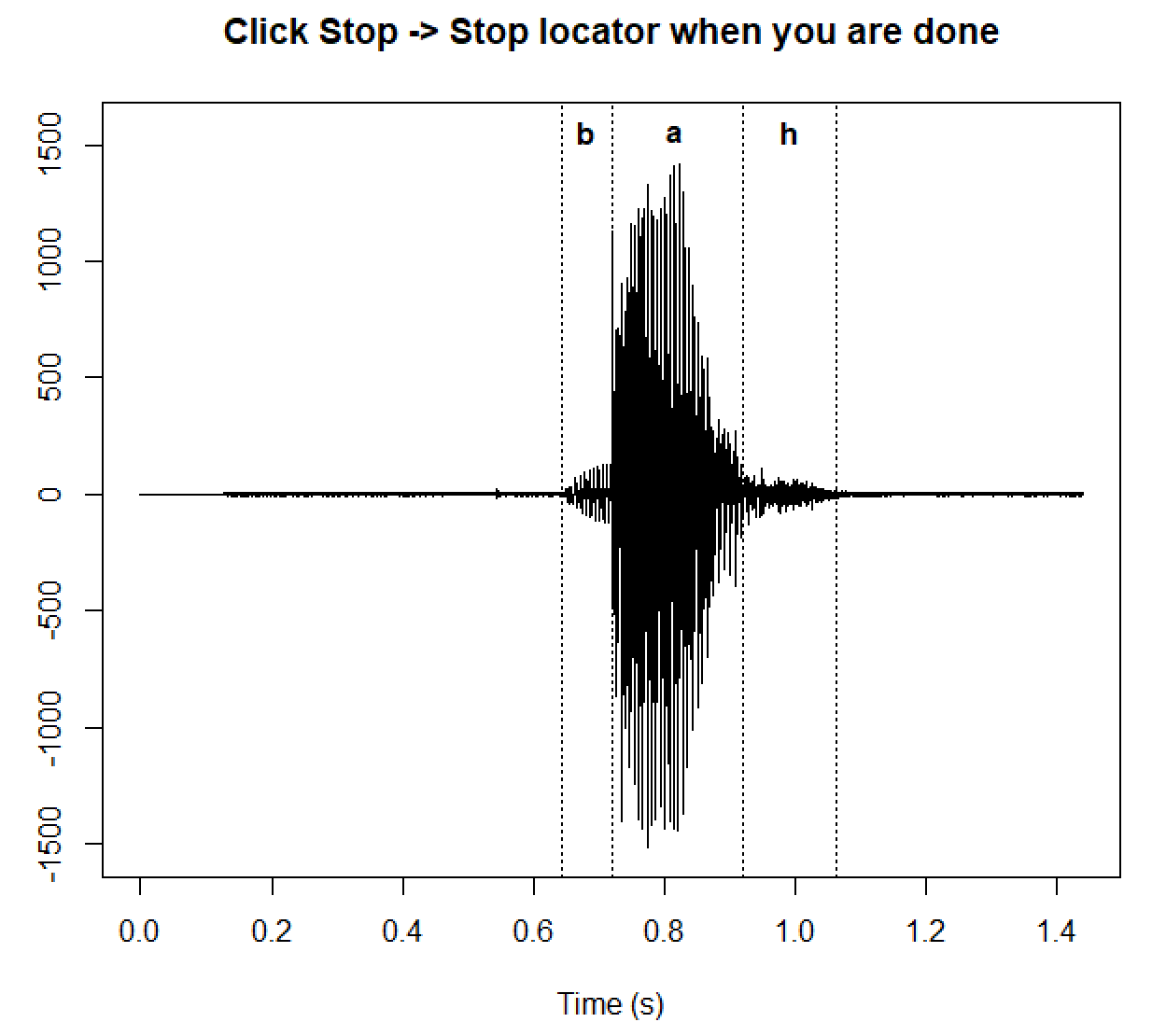
Next up, I will be asked to input the text for labels. I put in b, a, and h. This prompts the following text in the console:

Check the resulting annotation and type enter!

And the graphics device window will now also show the text:

This process will loop through however many annotation tiers you choose. When you’re done, the object new_tg (or whatever you choose to name it) will be saved in your environment. You can use this object when making a regular praatpicture figure, by passing it to the tg_obj argument:

praatpicture('ex/index.wav',
             tg_obj = new_tg)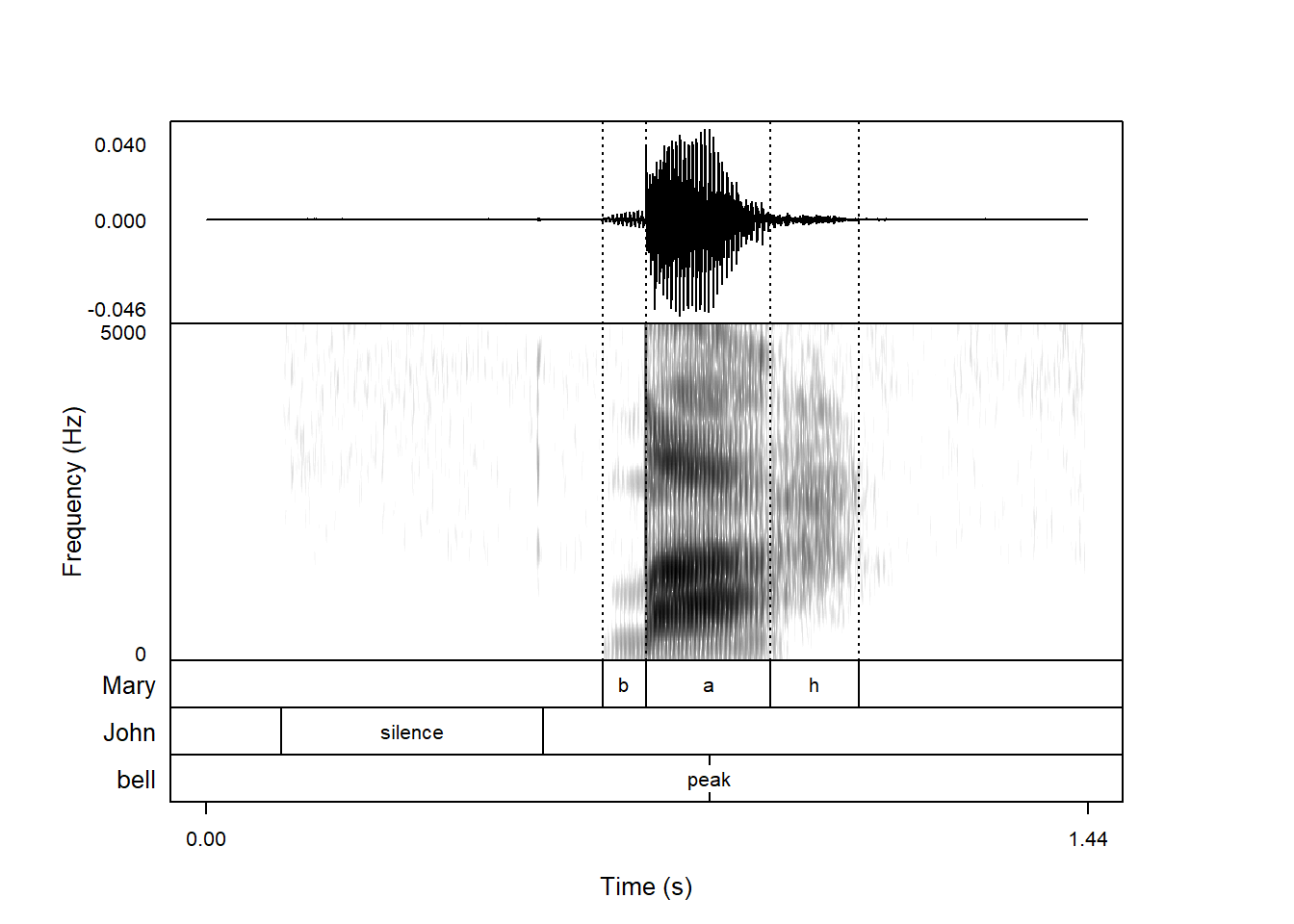

This now functions as a regular TextGrid!

If you want to make annotations like this but you’re working with a larger sound file and don’t want to show all of it, you can use the start and end arguments to show just part o fthe sound file (as when plotting with praatpicture).

11.2 Showing the spectrogram

If you prefer annotating on the basis of the spectrogram, you can do this by setting the show argument to 'spectrogram':

new_tg <- make_TextGrid('ex/index.wav',
                        tierNames = c('Mary', 'John', 'bell'),
                        show = 'spectrogram')

You will then see an image like this in the graphics window:

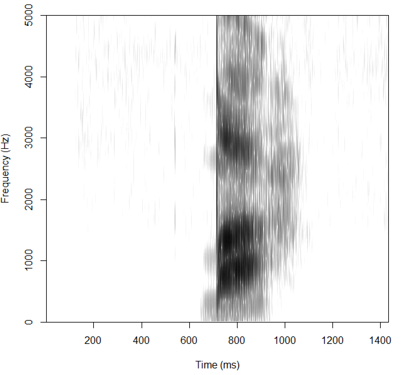
It otherwise works the same, but it is a fair bit slower since the spectrogram takes a while to generate.

11.3 Dynamically converting SAMPA to IPA

If you want to use IPA characters in your annotation but don’t want to go through the process of finding them, the argument sampa2ipa allows you to type in SAMPA transcriptions and convert them on the fly to IPA.

When I was making the first annotation tier of our sound file above and added the labels b, a, h, that was because I was lazy! These are actually a bilabial implosive, a low back vowel, and a voiced glottal fricative. I just didn’t want to find those symbols. I can do this easily with sampa2ipa set to TRUE:

new_tg_ipa <- make_TextGrid('ex/index.wav',
                            tierNames = 'IPA',
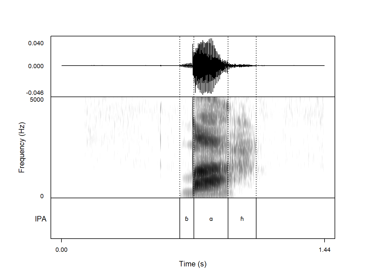
                            sampa2ipa = TRUE)

This time, I put boundaries in roughly the same locations as above, and when prompted, I will type b_<, A, and h\, which is the sampa way to annotate these sounds. When prompted to check the resulting annotation, I will now see the following:

If I use the resulting object with praatpicture(), the annotations will be in IPA:

praatpicture('ex/index.wav',
             tg_obj = new_tg_ipa)