praatpicture('ex/tg.wav',
             frames = c('sound', 'spectrogram'),
             proportion = c(30,70),
             wave_color = 'grey',
             spec_freqRange = c(200,10000))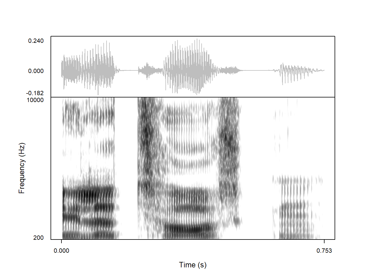
The spectrograms produced by praatpicture are by default similar to those produced by Praat, but users have a lot of options regarding both the general appearance of spectrograms and the underlying signal processing. We’ll cover those options here.
The spectrogram by default shows a frequency range between 0–5,000 Hz. The frequency range can be controlled with the spec_freqRange argument. For example, here we’ve removed the lowest frequencies (< 200 Hz), and extended the upper range to 10,000 Hz. This can be useful when you want to see what’s going on with sibilant-like sounds!
praatpicture('ex/tg.wav',
frames = c('sound', 'spectrogram'),
proportion = c(30,70),
wave_color = 'grey',
spec_freqRange = c(200,10000))
In addition to controlling the frequency range, there are also a few different frequency scales available in a different to raw Hertz. These can be selected with the spec_scale argument. Available scales are logged Hertz, the equivalent rectangular bandwidth scale and the Mel scale, using 1,000 Hz as the corner frequency as suggested by Gunnar Fant (1968). Log-Hz spectrograms don’t look great, but ERB-scaled and Mel-scaled spectrograms are quite useful – both of these involve transformations of the frequency range to closer resemble the auditory frequency response of humans. Be aware that plotting spectrograms in scales other than linear Hertz takes a fair bit longer (this is due to low-level details of how they’re implemented by the R plotting engine).
This is an ERB-scaled spectrogram:
praatpicture('ex/tg.wav',
             frames = c('sound', 'spectrogram'),
             proportion = c(30,70),
             wave_color = 'grey',
             spec_scale = 'erb')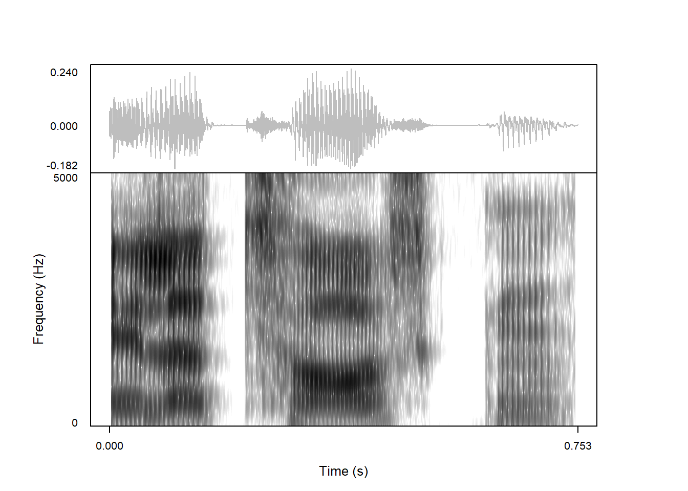
The default frequency range for ERB-scaled spectrograms is between 0.8–42, which corresponds roughly to the limits of the human frequency response (equivalent to 20–20,000 Hz). Note that this doesn’t work so well for the above example, since the sampling rate of the sound file is below 20,000 Hz.
This is a Mel-scaled spectrogram:
praatpicture('ex/tg.wav',
             frames = c('sound', 'spectrogram'),
             proportion = c(30,70),
             wave_color = 'grey',
             spec_scale = 'mel',
             spec_freqRange = c(0,3500))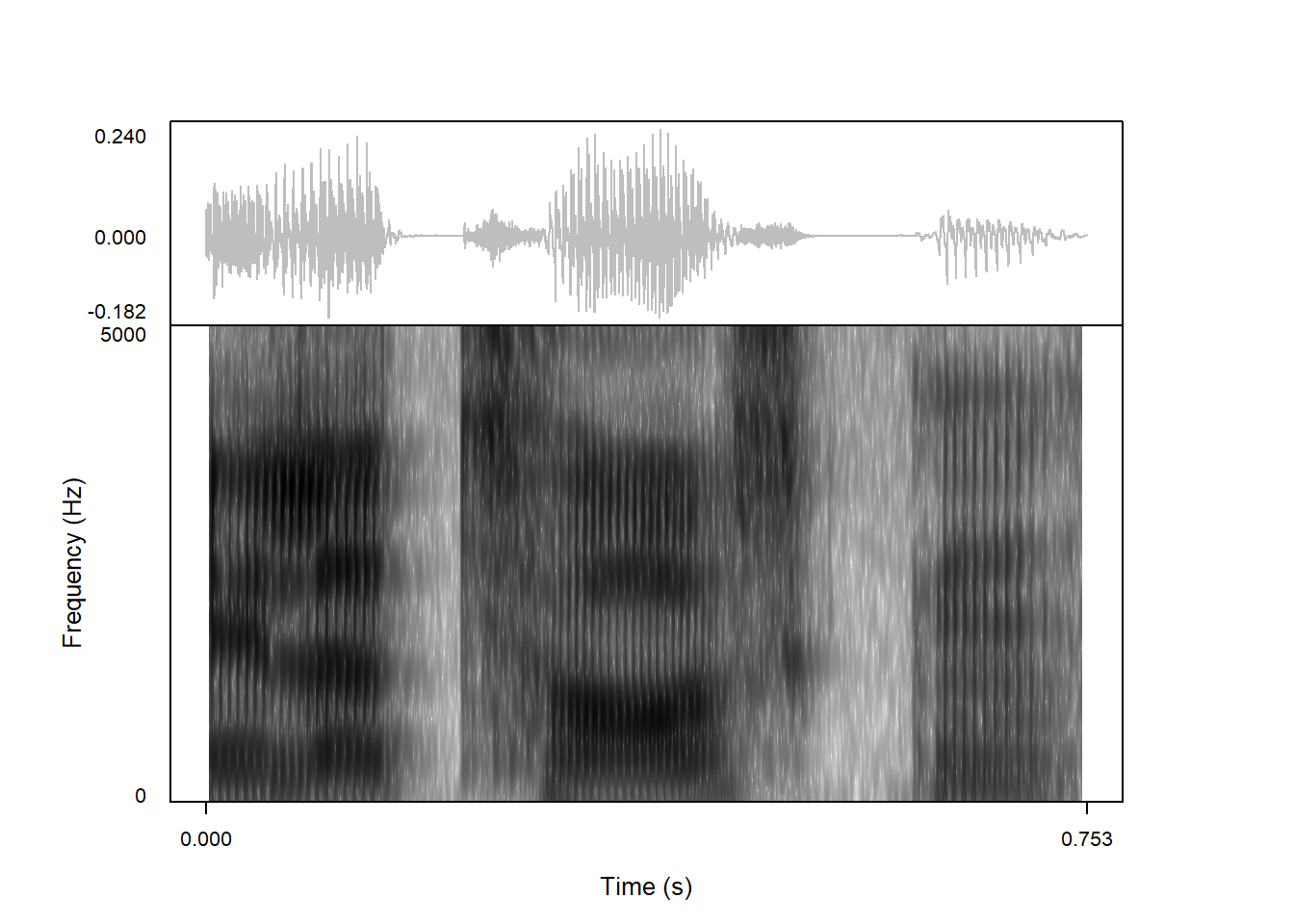
As with ERB-scaled spectrograms, Mel-scaled spectrograms by default have a frequency range corresponding roughly to the human frequency response, i.e. 4,400 Mel. This one goes only to 3,500 Mel, which is close to 10,000 Hz.
The dynamic range of the spectrogram is set to 50 dB by default, meaning that energy below 50 dB under the maximum amplitude in the spectrogram is rendered as white. This can be controlled with the spec_dynamicRange argument. The current Praat default is actually a bit higher, namely 70 dB, as shown here:
praatpicture('ex/tg.wav',
             frames = c('sound', 'spectrogram'),
             proportion = c(30,70),
             wave_color = 'grey',
             spec_dynamicRange = 70)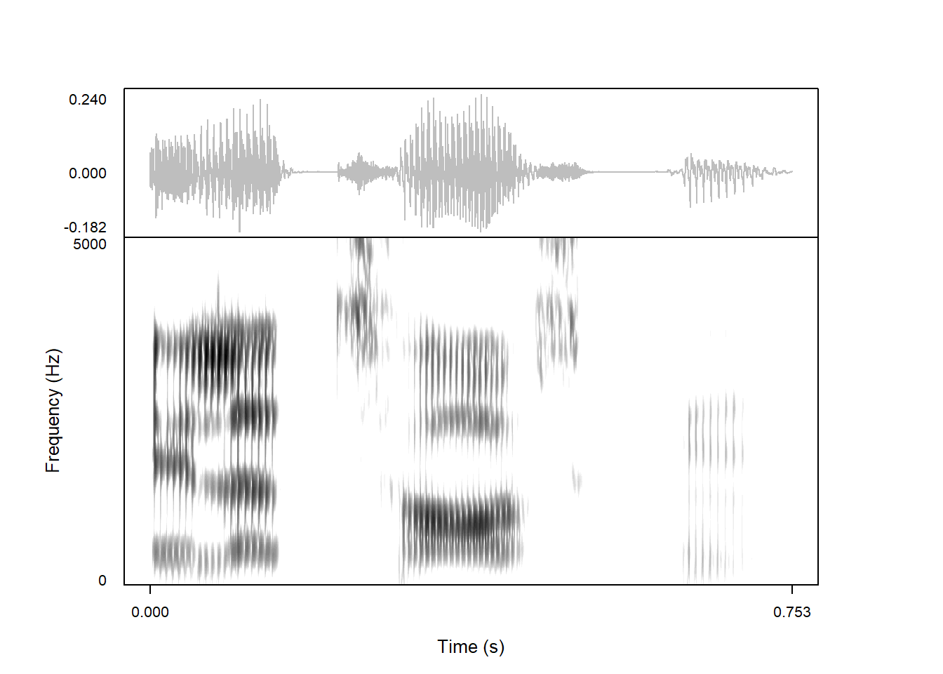
A very high dynamic range will give a spectrogram without any white areas:
praatpicture('ex/tg.wav',
             frames = c('sound', 'spectrogram'),
             proportion = c(30,70),
             wave_color = 'grey',
             spec_dynamicRange = 150)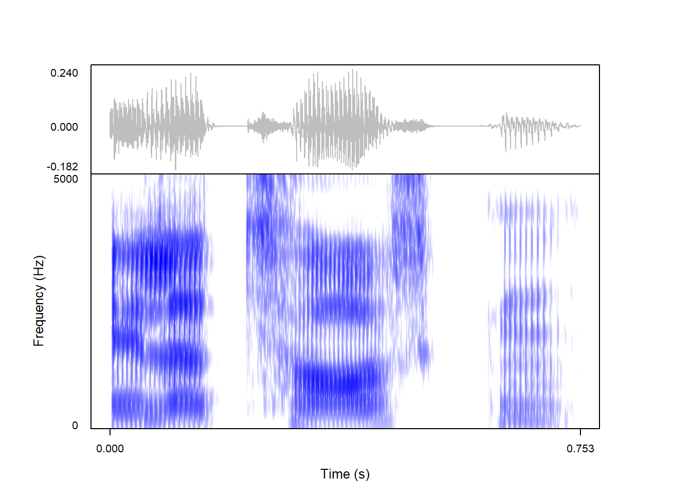
And with a very low dynamic range, only areas with very high energy is shown:
praatpicture('ex/tg.wav',
             frames = c('sound', 'spectrogram'),
             proportion = c(30,70),
             wave_color = 'grey',
             spec_dynamicRange = 30)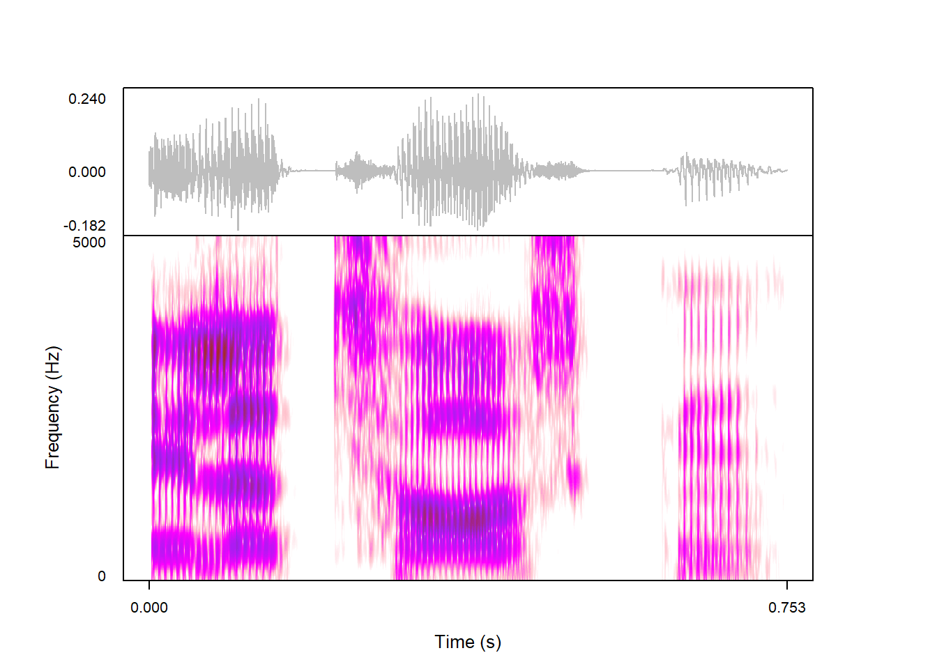
By default, areas of the specrogram with low energy are rendered in white and areas with energy in black. This is controlled with the spec_color argument, which should be at least two colors. For example, you could render high frequencies in blue like so:
praatpicture('ex/tg.wav',
             frames = c('sound', 'spectrogram'),
             proportion = c(30,70),
             wave_color = 'grey',
             spec_color = c('white', 'blue'))
It is also possible to use more complicated color schemes, by specifying both the color used for lowest values, highest values, and any number of in-between values. For example, this plot uses brown for high values, white for low values, and a bunch of pink-ish hues for in-between values
praatpicture('ex/tg.wav',
             frames = c('sound', 'spectrogram'),
             proportion = c(30,70),
             wave_color = 'grey',
             spec_color = c('white', 'pink', 'magenta', 'purple', 'brown'))
The label along the y-axis says Frequency (Hz) by default. This is controlled with the spec_axisLabel argument; here’s one that just says Spectrogram:
praatpicture('ex/tg.wav',
             frames = c('sound', 'spectrogram'),
             proportion = c(30,70),
             wave_color = 'grey',
             spec_axisLabel = 'Spectrogram')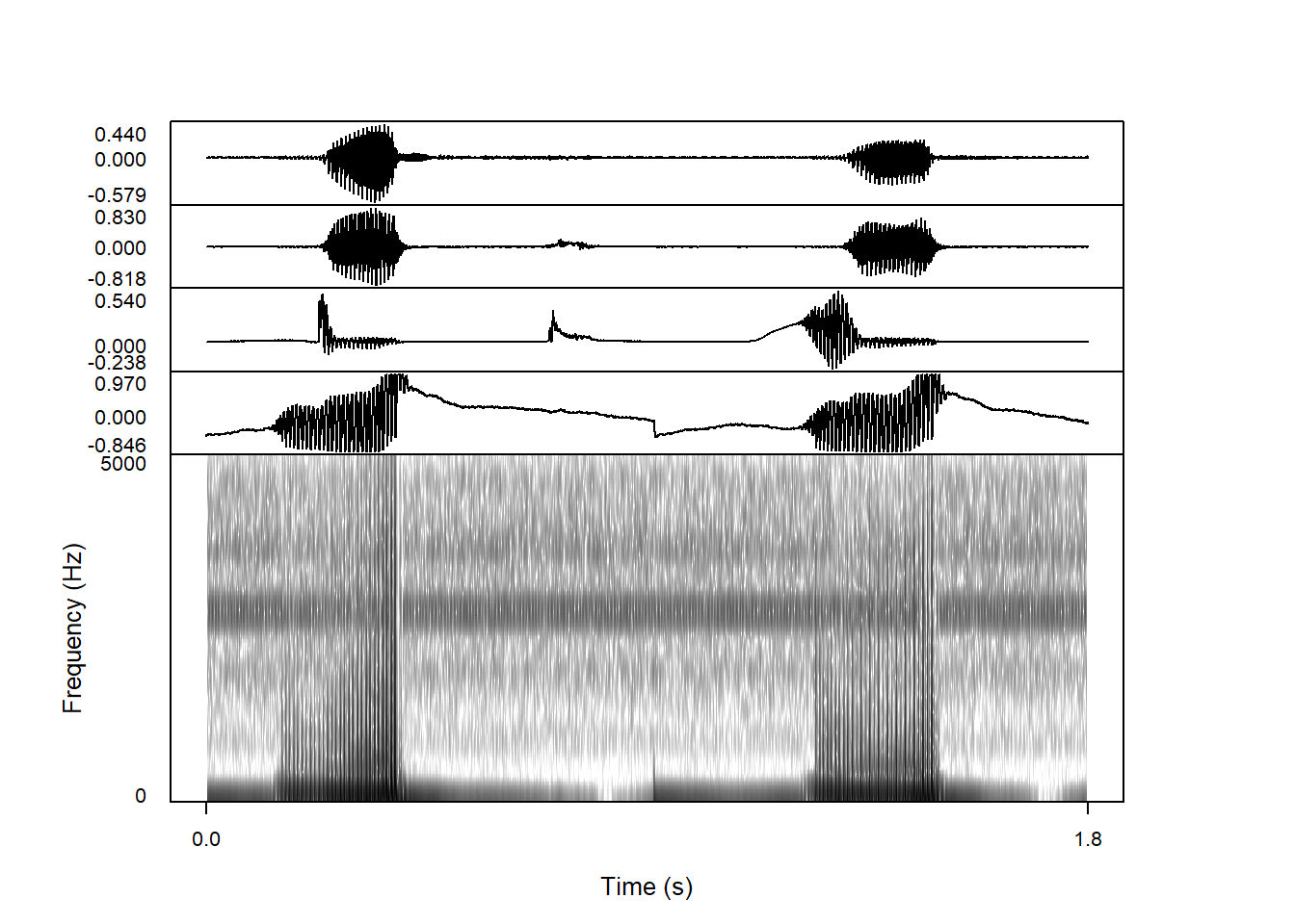
When plotting multi-channel data, the spectrogram is always based on one of the channels. By default it is the first one, as shown here:
praatpicture('ex/multichannel.wav',
             start = 0.6, end = 2.4,
             frames = c('sound', 'spectrogram'))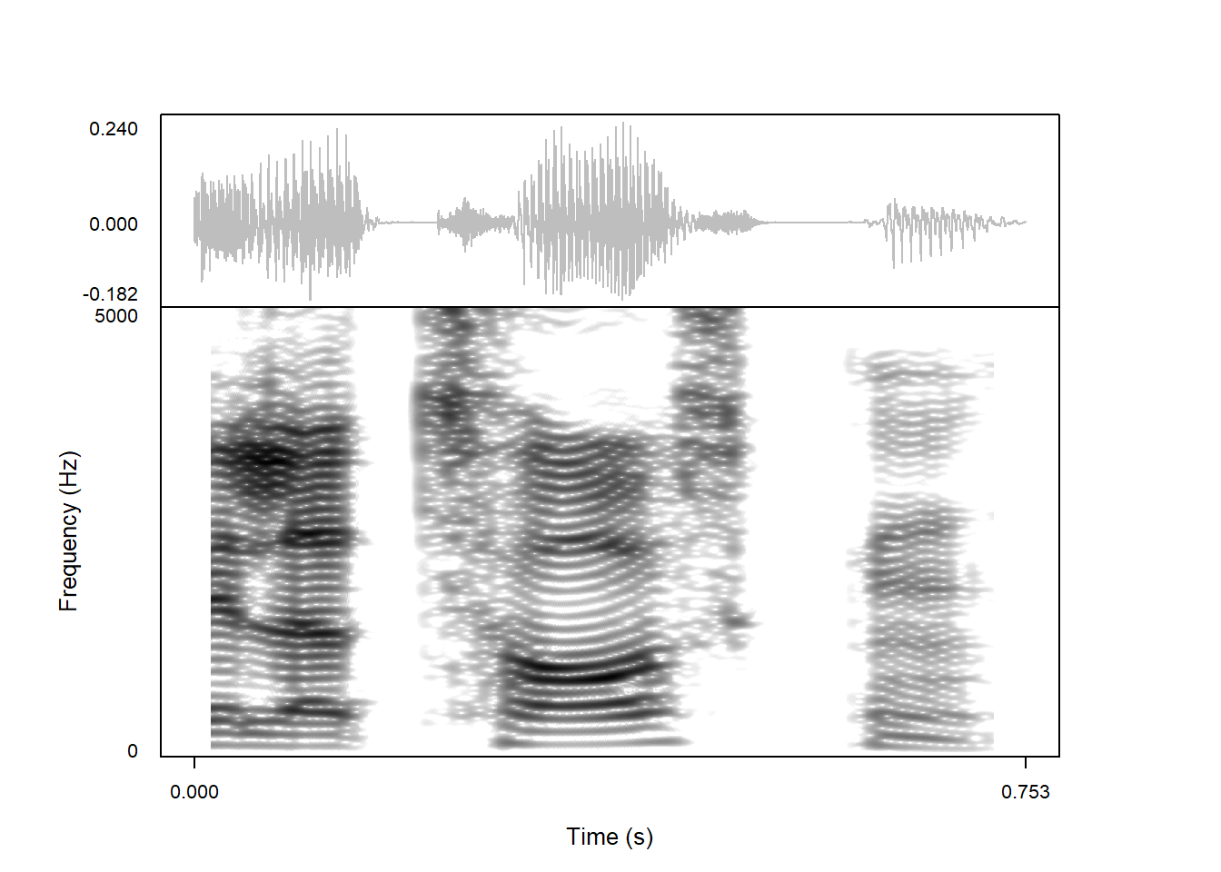
If we were interested in using a different channel for the spectrogram, the spec_channel argument can be used for that purpose. Here’s a spectrogram showing the intraoral pressure signal:
praatpicture('ex/multichannel.wav',
             start = 0.6, end = 2.4,
             frames = c('sound', 'spectrogram'),
             spec_channel = 4)
The default window length used for generating spectra is 5 ms, following Praat. This gives you a narrowband spectrogram. Window length is controlled with the spec_windowLength argument. For example, using 30 ms will give you a broadband spectrogram. This has lower temporal resolution, but is great for seeing the harmonics!
praatpicture('ex/tg.wav',
             frames = c('sound', 'spectrogram'),
             proportion = c(30,70),
             wave_color = 'grey',
             spec_windowLength = 0.03)
Spectra are generated with Gaussian windows by default, but a range of other shapes are available. A bunch of other options are available, although the difference between most of them is marginal. Gaussian window shapes are a bit slower, but the difference is small enough that it should make a difference for most users.
This uses Hamming windows:
praatpicture('ex/tg.wav',
             frames = c('sound', 'spectrogram'),
             proportion = c(30,70),
             wave_color = 'grey',
             spec_windowShape = 'Hamming')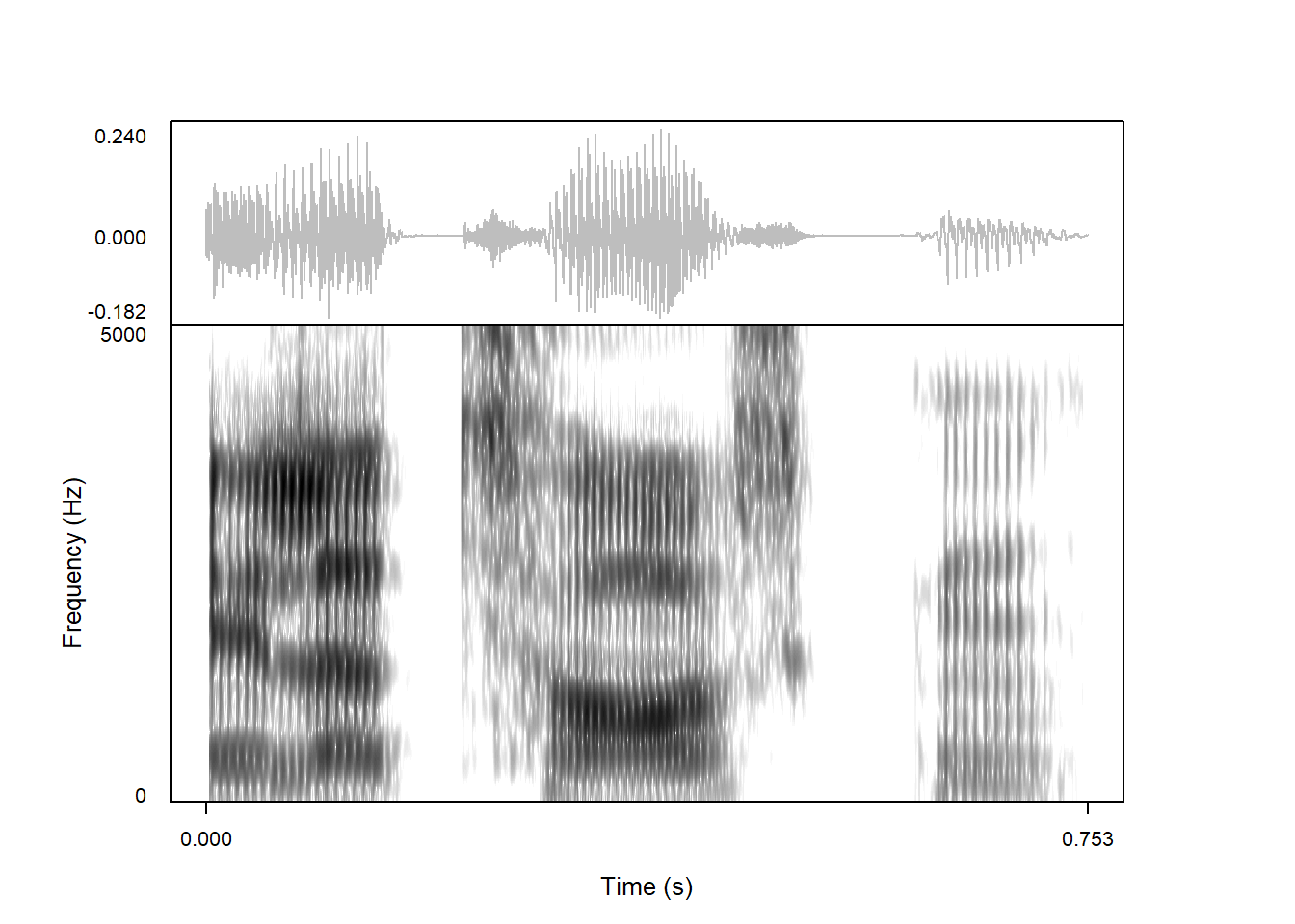
Hanning windows:
praatpicture('ex/tg.wav',
             frames = c('sound', 'spectrogram'),
             proportion = c(30,70),
             wave_color = 'grey',
             spec_windowShape = 'Hanning')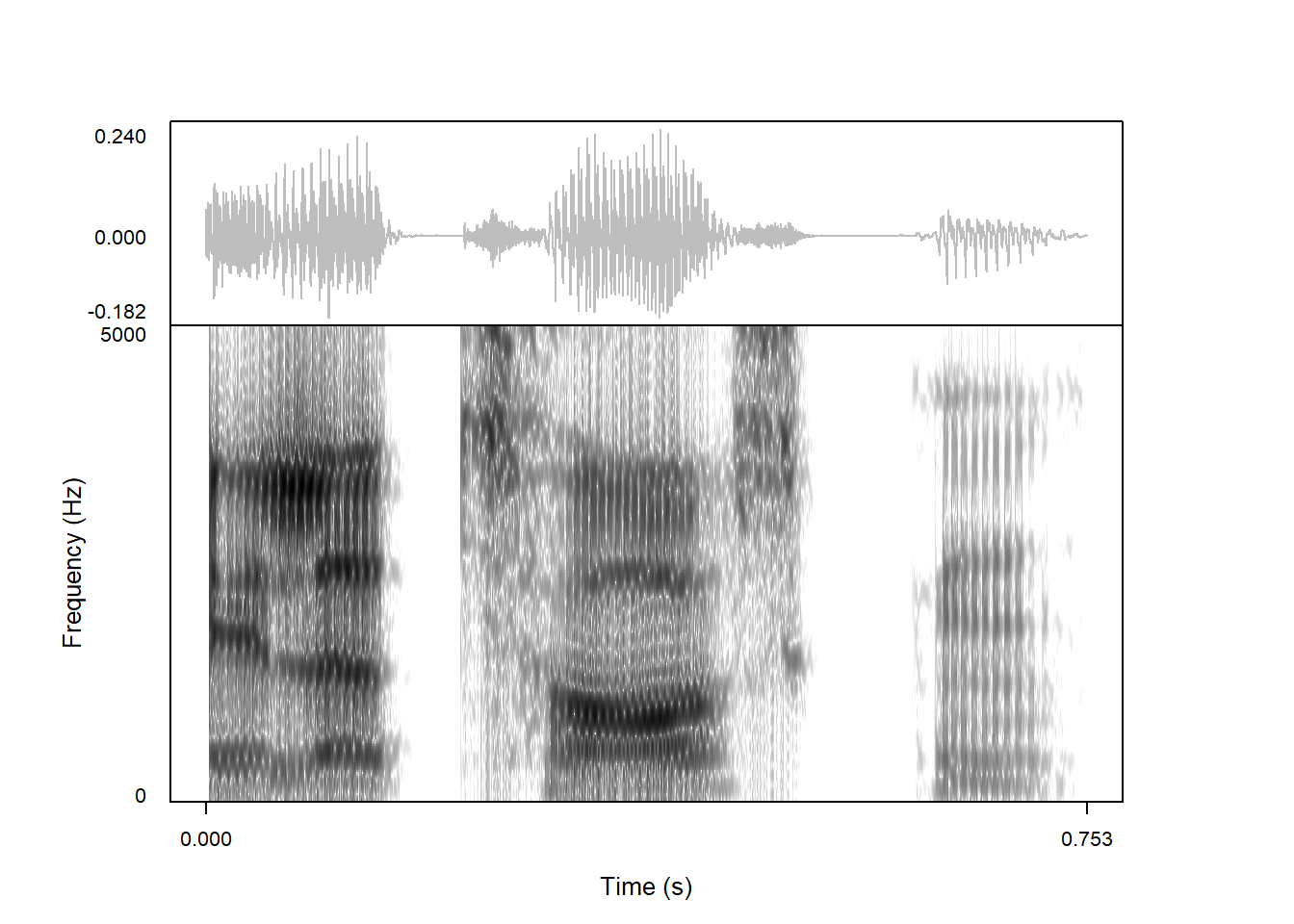
Bartlett windows:
praatpicture('ex/tg.wav',
             frames = c('sound', 'spectrogram'),
             proportion = c(30,70),
             wave_color = 'grey',
             spec_windowShape = 'Bartlett')
And here square (or ‘rectangular’) windows, which is equivalent to an un-edited window. These spectrograms clearly look worse:
praatpicture('ex/tg.wav',
             frames = c('sound', 'spectrogram'),
             proportion = c(30,70),
             wave_color = 'grey',
             spec_windowShape = 'square')
Finally, this uses Blackman windows:
praatpicture('ex/tg.wav',
             frames = c('sound', 'spectrogram'),
             proportion = c(30,70),
             wave_color = 'grey',
             spec_windowShape = 'Blackman')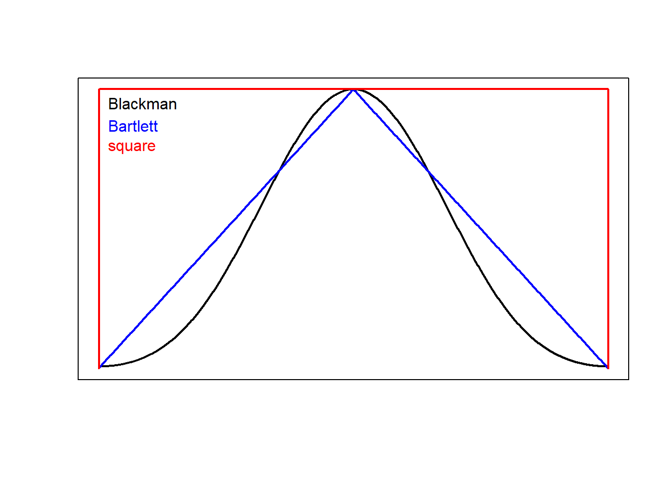
Typically you don’t need to! The Praat documentation says that window shapes other than Gaussian are included for “pedagogical purposes” only. When plotting spectrograms of speech sounds, it typically won’t matter much if you use Gaussian, Hanning, or Hamming windows, as they have very similar shapes. These windows look like this:
Gaussian_window <- phonTools::windowfunc(1000, type = 'gaussian')
Hann_window <- phonTools::windowfunc(1000, type = 'hann')
Hamming_window <- phonTools::windowfunc(1000, type = 'hamming')

plot(Gaussian_window, type = 'l', xaxt = 'n', yaxt = 'n', xlab = '', ylab = '',
     ylim = c(-0, 1), lwd = 2)
lines(Hann_window, col = 'blue', lwd = 2)
lines(Hamming_window, col = 'red', lwd = 2)
text(0, 1, labels = 'Gaussian', adj = 0)
text(0, 0.92, labels = 'Hanning', adj = 0, col = 'blue')
text(0, 0.84, labels = 'Hamming', adj = 0, col = 'red')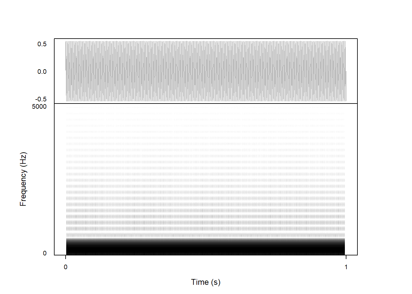
These are all variations on the same idea, smooth functions that allow most of the information at the center of a window to pass through and less information at the edges. Bartlett windows can also be considered a variation on the same general idea, only they are pyramid-shaped rather than smooth, while square windows simply allow all information to pass through. Blackman windows are also smooth – these are not available in Praat, but are available in the phonTools library that are used to generate spectrograms in praatpicture.
Blackman_window <- phonTools::windowfunc(1000, type = 'blackman')
Bartlett_window <- phonTools::windowfunc(1000, type = 'bartlett')
square_window <- c(0, phonTools::windowfunc(998, type = 'rectangular'), 0)

plot(Blackman_window, type = 'l', xaxt = 'n', yaxt = 'n', xlab = '', ylab = '',
     ylim = c(-0, 1), lwd = 2)
lines(Bartlett_window, col = 'blue', lwd = 2)
lines(square_window, col = 'red', lwd = 2)
text(20, 0.95, labels = 'Blackman', adj = 0)
text(20, 0.87, labels = 'Bartlett', adj = 0, col = 'blue')
text(20, 0.79, labels = 'square', adj = 0, col = 'red')
The argument for relying on Gaussian window shapes in Praat is that they are supposedly the only window shape that doesn’t produce so-called sidelobes when plotting a simple sine wave. A spectrogram showing a 200 Hz sine wave should show only a horizontal line near 200 Hz, but you may also see vertical stripes in the spectrogram that are an artefact of the window shape, and do not indicate anything present in the signal. For example, here is a spectrogram of a 1-second 200 Hz sine wave.
praatpicture('ex/simple.wav', frames = c('sound', 'spectrogram'),
             proportion = c(30,70),
             wave_color = 'grey',
             spec_windowShape = 'Hamming')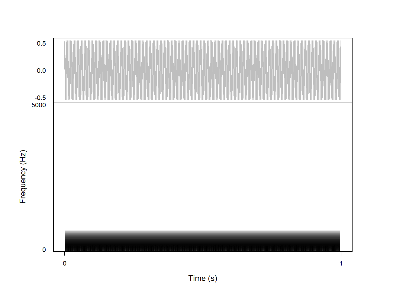
Unfortunately, when plotting spectrograms using the Gaussian window shapes available in the phonTools package, sidelobes are also visible in the spectrogram, although they are less prominent:
praatpicture('ex/simple.wav', frames = c('sound', 'spectrogram'),
             proportion = c(30,70),
             wave_color = 'grey',
             spec_windowShape = 'Gaussian')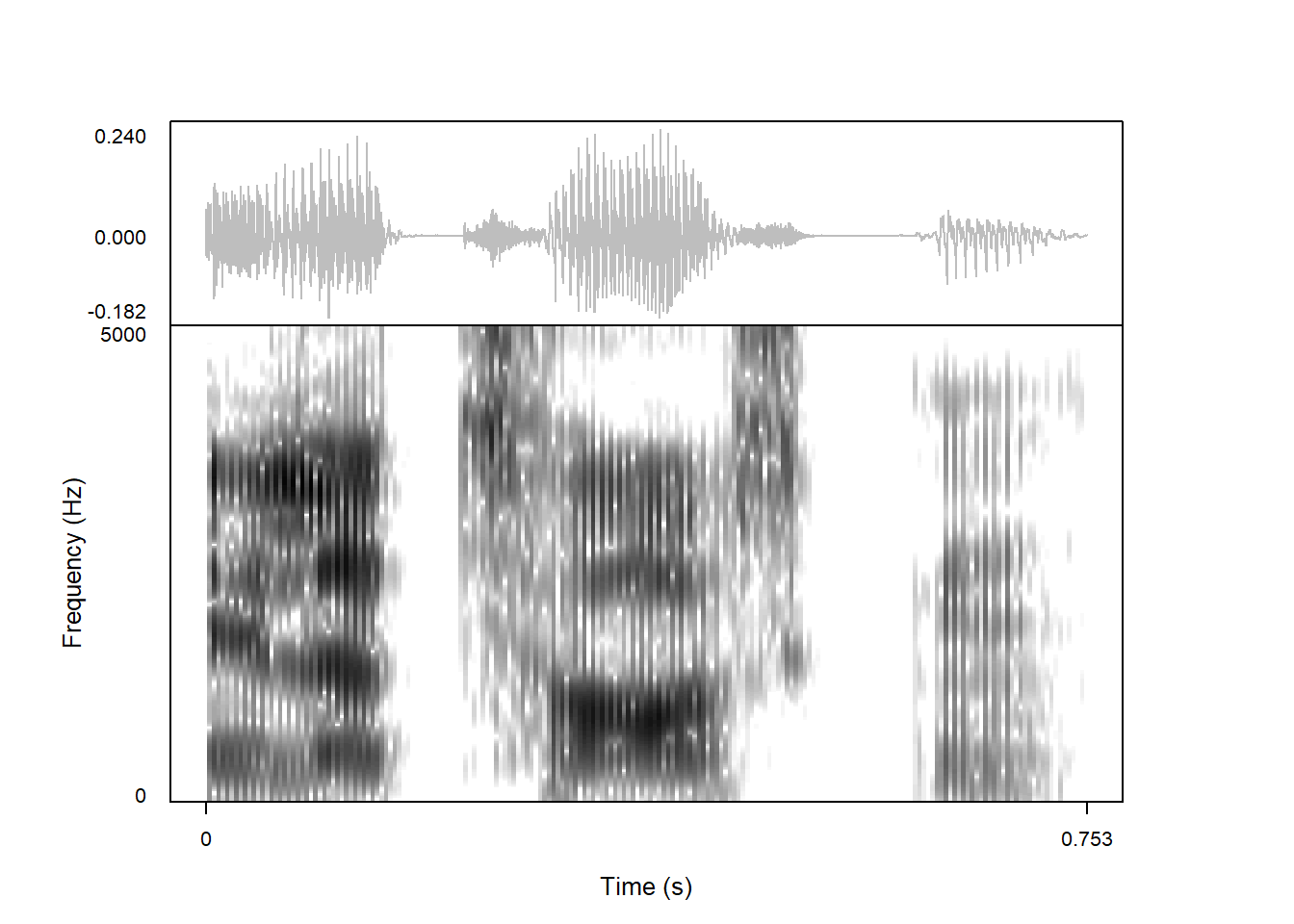
This does not happen in Praat, and must mean that the phonTools Gaussian window shapes are not the same as those used by Praat. This is a mystery I have yet to solve, and this is why praatpicture also supports Blackman windows, because they do not have these artefacts:
praatpicture('ex/simple.wav', frames = c('sound', 'spectrogram'),
             proportion = c(30,70),
             wave_color = 'grey',
             spec_windowShape = 'Blackman')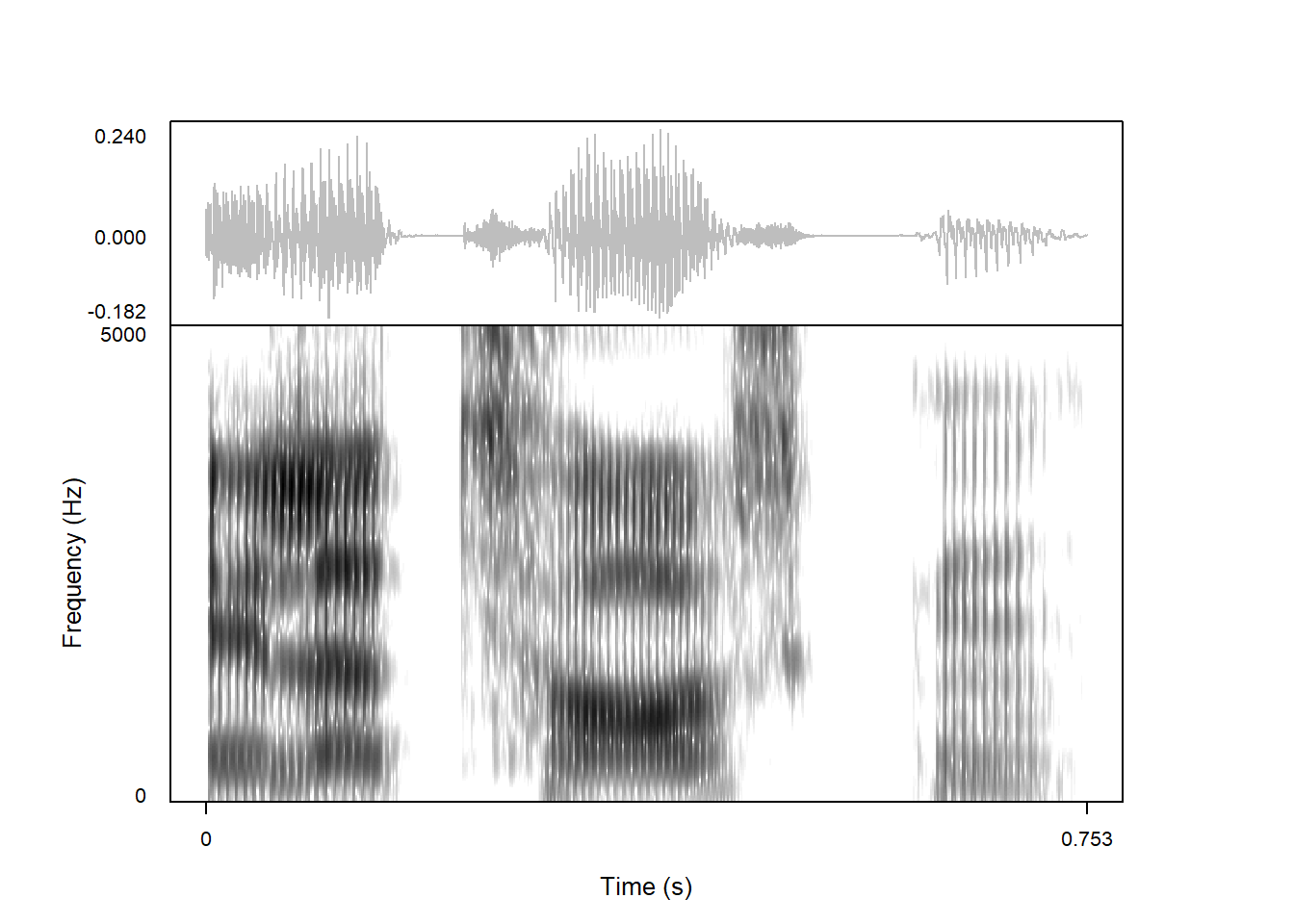
By default, spectrograms are composed of 1,000 spectral slices. This is controlled with the spec_timeStep argument. Lowering this will speed up generating the spectrogram, but the spectrogram will likely look pixellated. Here is one composed from “only” 200 spectral slices:
praatpicture('ex/tg.wav',
             frames = c('sound', 'spectrogram'),
             proportion = c(30,70),
             wave_color = 'grey',
             spec_timeStep = 200)
500 spectral slices will usually be enough to render a spectrogram that doesn’t look pixellated, and will also speed up generating the spectrogram a fair bit.
praatpicture('ex/tg.wav',
             frames = c('sound', 'spectrogram'),
             proportion = c(30,70),
             wave_color = 'grey',
             spec_timeStep = 500)
If you’re printing a really large plot, that might not be enough though. 1,000 is enough for most purposes, but again, if you’re printing something very large, you may want to set a higher time step.