praatpicture('ex/ex.wav',
             frames = c('sound', 'pitch'),
             proportion = c(30,70),
             wave_color = 'grey')
The pitch tracks plotted by praatpicture by default look similar to those produced by Praat, but users have a lot of options regarding both the general appearance of pitch tracks and the underlying signal processing, or to capitalize on the signal processing provided by Praat (see Section 6.3). We’ll cover those options here.
When plotting pitch in Praat, pitch tracks are either ‘drawn’ or ‘speckled’. The default is ‘drawn’, i.e. line plots:
praatpicture('ex/ex.wav',
frames = c('sound', 'pitch'),
proportion = c(30,70),
wave_color = 'grey')
This can be controlled with the pitch_plotType argument. A ‘speckled’ plot will draw points for the individual pitch measures:
praatpicture('ex/ex.wav',
             frames = c('sound', 'pitch'),
             proportion = c(30,70),
             wave_color = 'grey',
             pitch_plotType = 'speckle')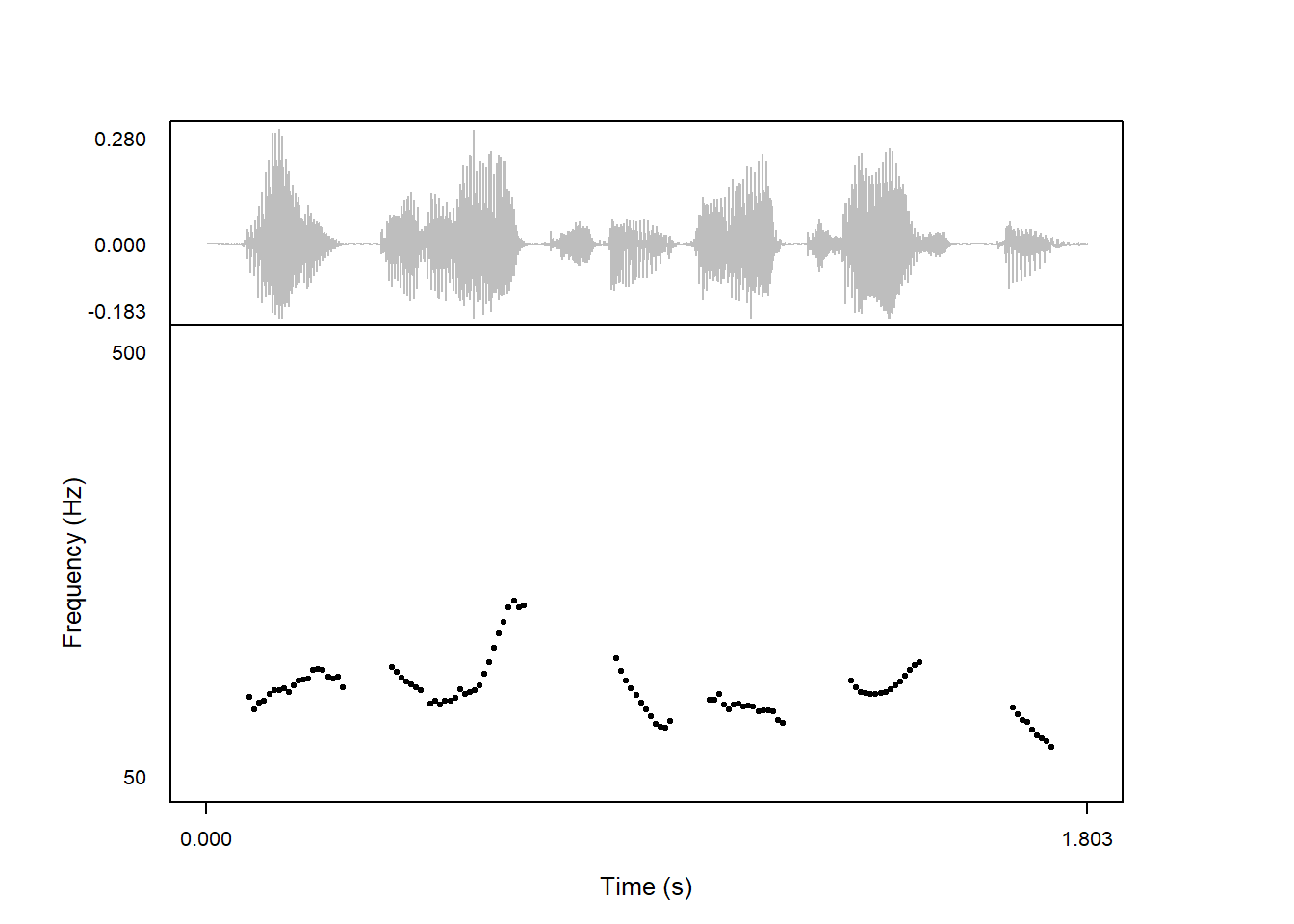
If you want to draw a pitch contour with a thicker line, you can set the drawSize argument larger than 1 (which will also affect other drawn derived signals, i.e. formants or intensity).
praatpicture('ex/ex.wav',
             frames = c('sound', 'pitch'),
             proportion = c(30,70),
             wave_color = 'grey',
             drawSize = 3)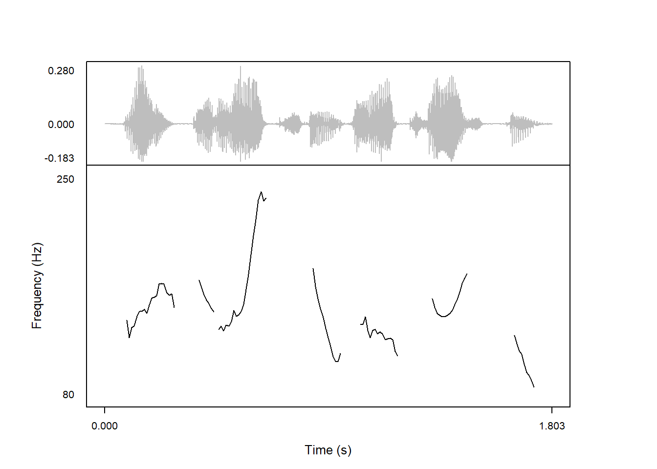
The speckleSize argument works similarly if you want larger points in a speckled plot.
praatpicture('ex/ex.wav',
             frames = c('sound', 'pitch'),
             proportion = c(30,70),
             wave_color = 'grey',
             pitch_plotType = 'speckle',
             speckleSize = 2)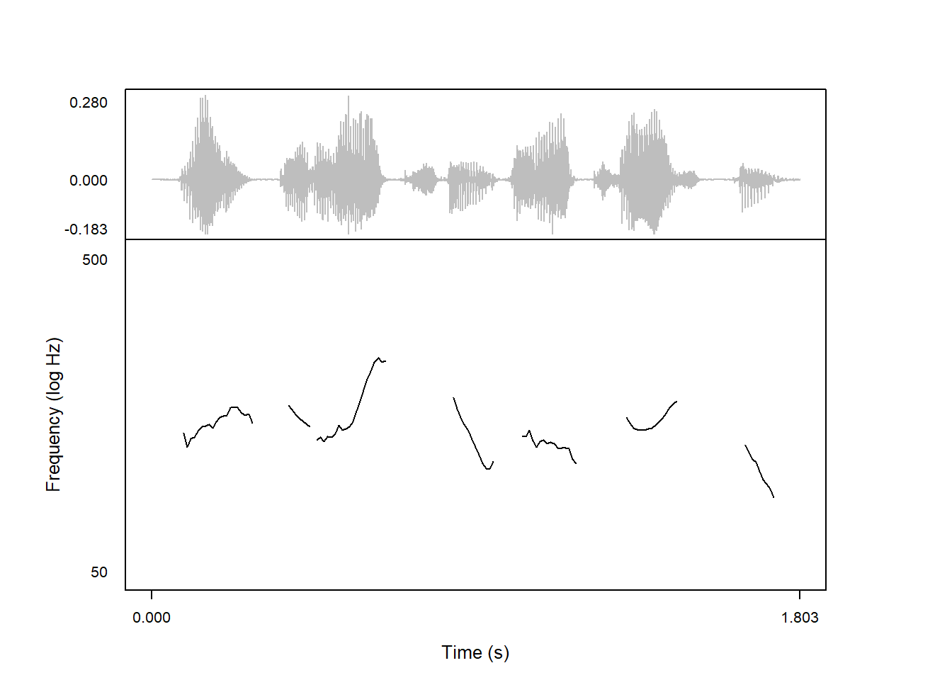
If you want smaller speckles, you can set speckleSize lower, e.g. 0.5.
The default frequency range for pitch plots shows between 50–500 Hz. This is rather broad for most purposes. Frequency range can be controlled with the pitch_freqRange argument. Here, a frequency range between 80–250 Hz is probably more suitable:
praatpicture('ex/ex.wav',
             frames = c('sound', 'pitch'),
             proportion = c(30,70),
             wave_color = 'grey',
             pitch_freqRange = c(80,250))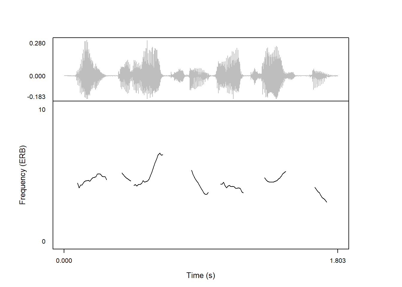
By default, pitch tracks are plotted in a raw frequency scale. A range of other options are available for scaling the pitch values. This is controlled with the pitch_scale argument.
log or logarithmic will both produce a plot that is log-scaled on the y-axis.
praatpicture('ex/ex.wav',
             frames = c('sound', 'pitch'),
             proportion = c(30,70),
             wave_color = 'grey',
             pitch_scale = 'log')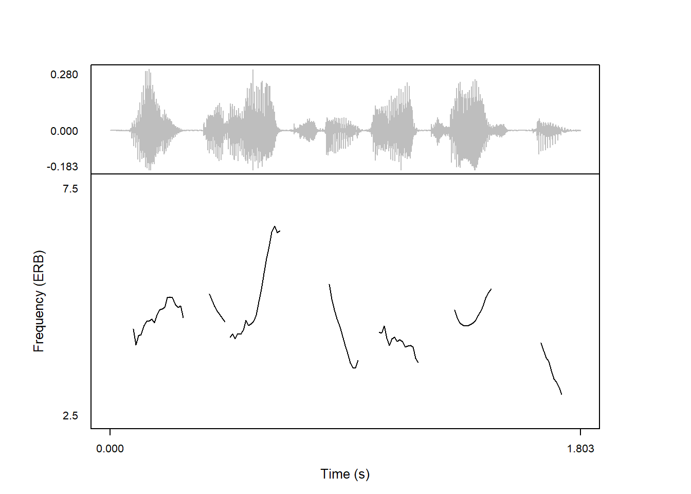
Notice that the y-axis label changes automatically to reflect the scale.
Other scales have different default frequency ranges. The equivalent rectangular bandwidth (ERB) scale by default goes from 1–10:
praatpicture('ex/ex.wav',
             frames = c('sound', 'pitch'),
             proportion = c(30,70),
             wave_color = 'grey',
             pitch_scale = 'erb')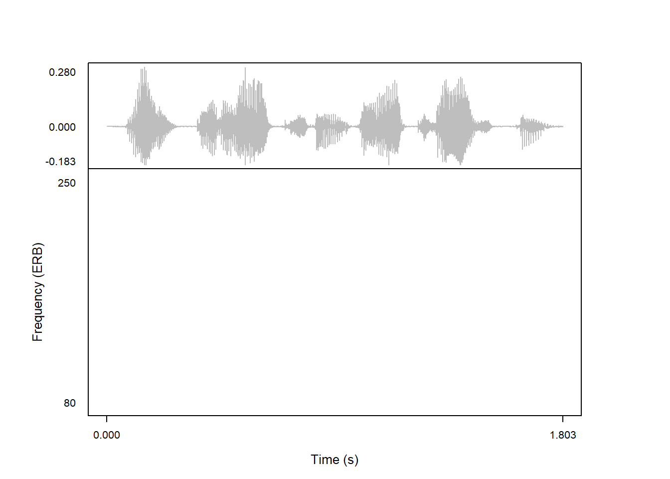
This can of course still be controlled, here is 2.5–7.5 for example:
praatpicture('ex/ex.wav',
             frames = c('sound', 'pitch'),
             proportion = c(30,70),
             wave_color = 'grey',
             pitch_freqRange = c(2.5,7.5),
             pitch_scale = 'erb')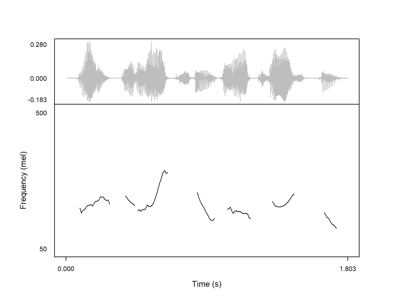
Although be careful that the frequency range fits with the scale. Setting a frequency range between, say, 80–250 (suitable for Hz) for an ERB-scaled plot will simply produce an empty plot:
praatpicture('ex/ex.wav',
             frames = c('sound', 'pitch'),
             proportion = c(30,70),
             wave_color = 'grey',
             pitch_freqRange = c(80,250),
             pitch_scale = 'erb')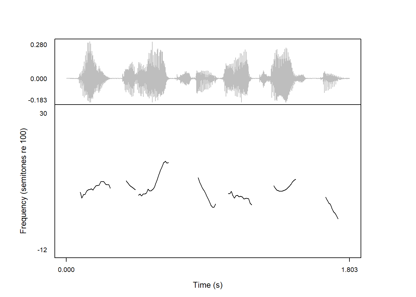
It is also possible to produce Mel-scaled plots:
praatpicture('ex/ex.wav',
             frames = c('sound', 'pitch'),
             proportion = c(30,70),
             wave_color = 'grey',
             pitch_scale = 'mel')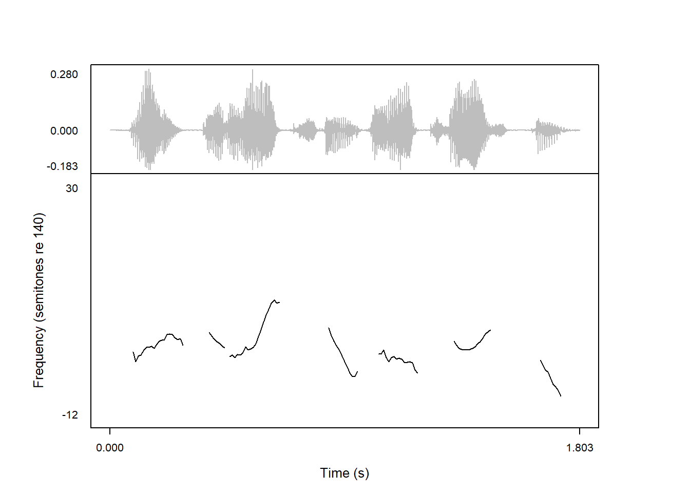
And finally semitones:
praatpicture('ex/ex.wav',
             frames = c('sound', 'pitch'),
             proportion = c(30,70),
             wave_color = 'grey',
             pitch_scale = 'semitones')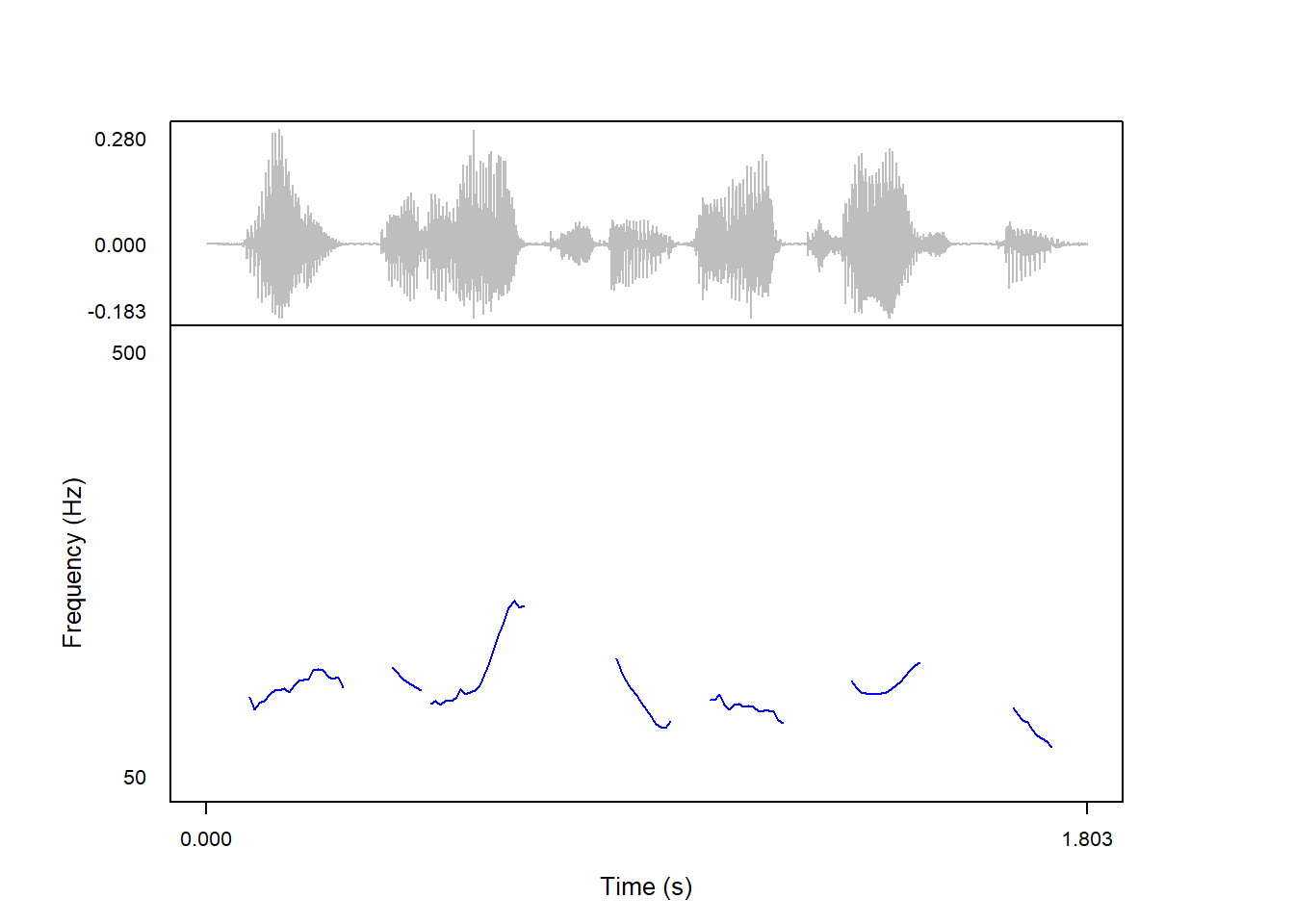
The default reference level for semitones is 100 Hz; this can be controlled with the pitch_semitonesRe argument. This speaker probably has a mean pitch closer to 140 Hz, so we could set the semitones reference to match that:
praatpicture('ex/ex.wav',
             frames = c('sound', 'pitch'),
             proportion = c(30,70),
             wave_color = 'grey',
             pitch_scale = 'semitones',
             pitch_semitonesRe = 140)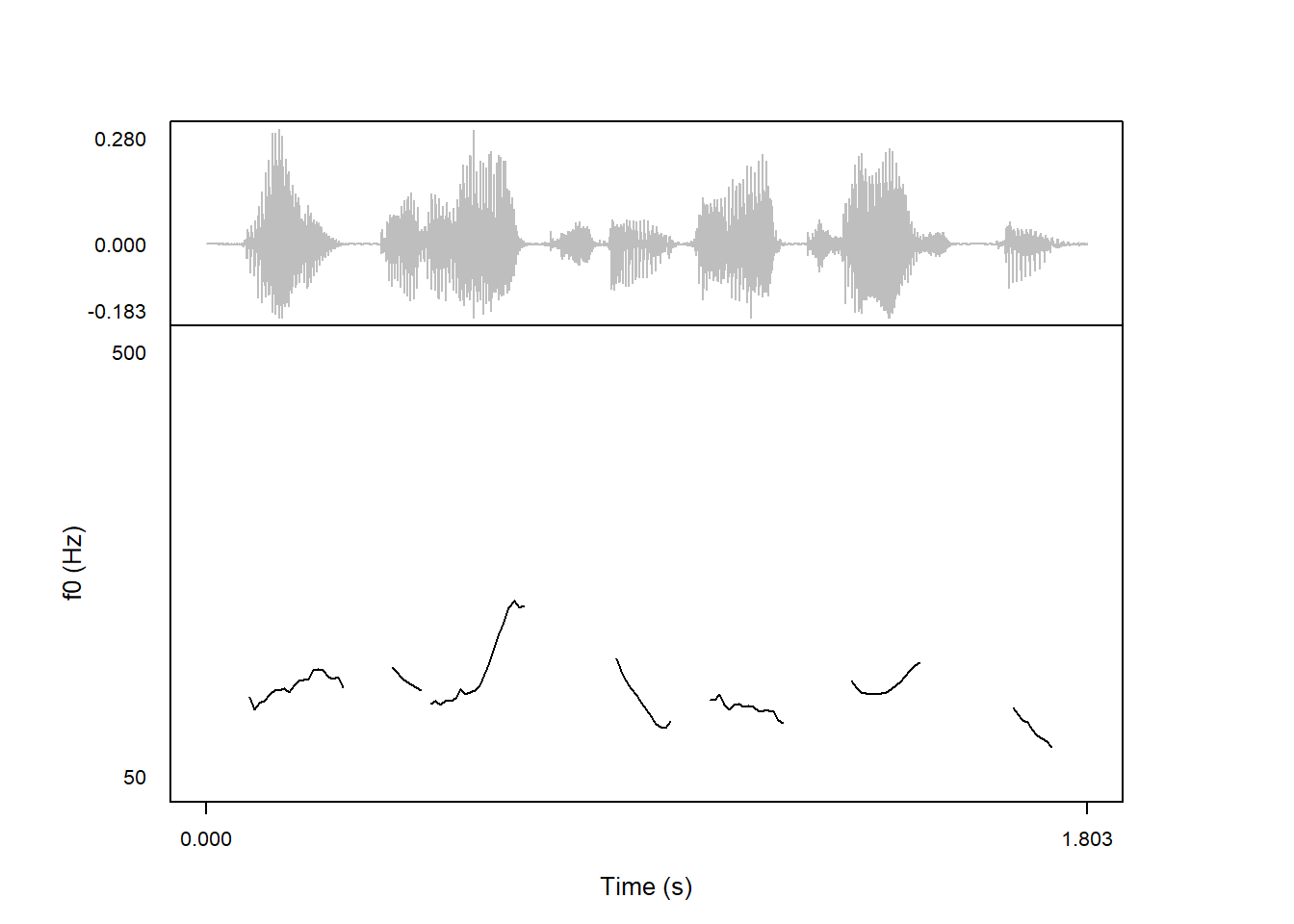
The color of the pitch trace is controlled with the pitch_color argument. Here’s a blue contour:
praatpicture('ex/ex.wav',
             frames = c('sound', 'pitch'),
             proportion = c(30,70),
             wave_color = 'grey',
             pitch_color = 'blue')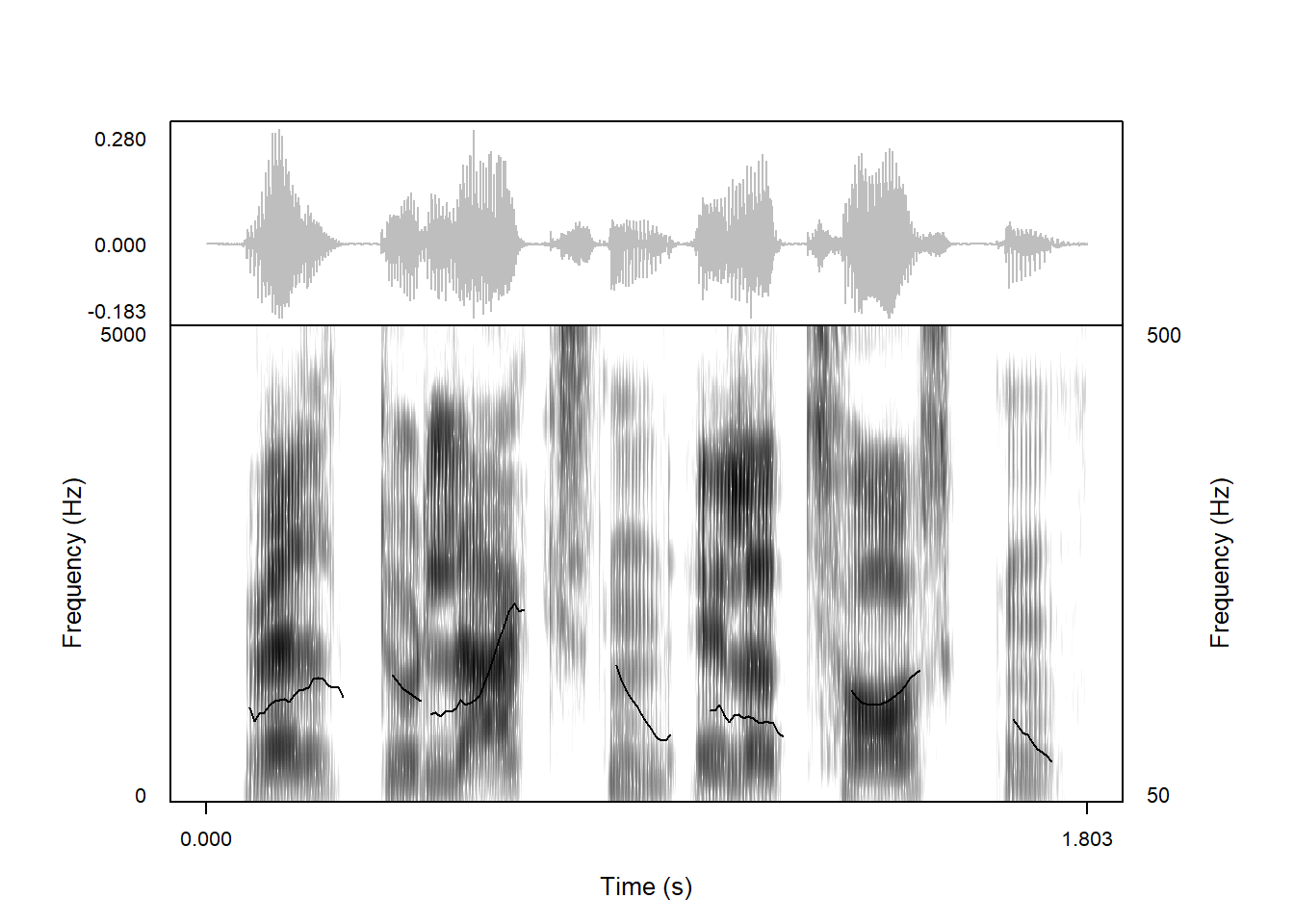
Some fancier coloring options are available when a pitch track is overlaid on spectrograms or waveforms; more on that in Section 6.1.6 and Section 6.2.
As we’ve seen above, the y-axis label for pitch plots is automatically adapted to different frequency scales. Users can also specify their own axis labels, using the pitch_axisLabel argument. For example, we might want to refer to it as f0:
praatpicture('ex/ex.wav',
             frames = c('sound', 'pitch'),
             proportion = c(30,70),
             wave_color = 'grey',
             pitch_axisLabel = 'f0 (Hz)')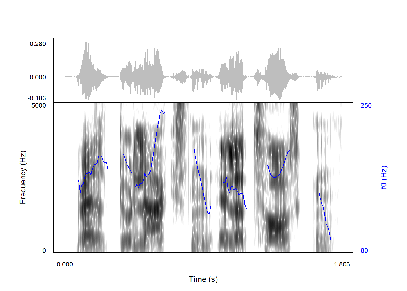
Instead of drawing pitch in its own frame, it is also possible to overlay a pitch contour on a spectrogram. In this case, pitch should not be specified as one of the frames; this is instead controlled with the Boolean pitch_plotOnSpec argument.
praatpicture('ex/ex.wav',
             frames = c('sound', 'spectrogram'),
             proportion = c(30,70),
             wave_color = 'grey',
             pitch_plotOnSpec = TRUE)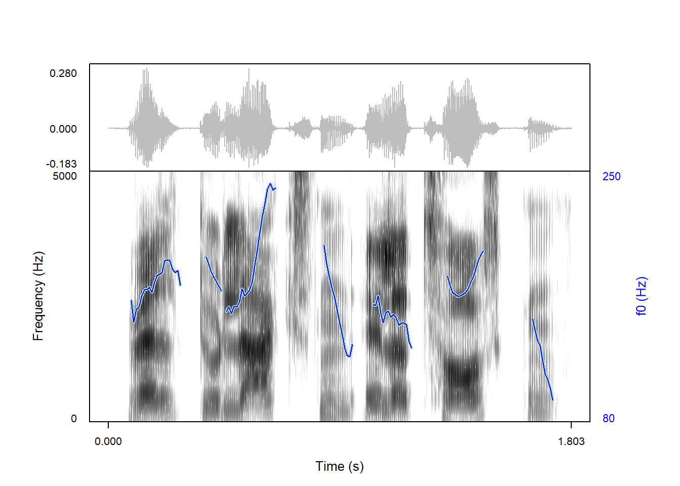
The other arguments controlling pitch appearance (and signal processing) also work when overlaying pitch on the spectrogram:
praatpicture('ex/ex.wav',
             frames = c('sound', 'spectrogram'),
             proportion = c(30,70),
             wave_color = 'grey',
             pitch_plotOnSpec = TRUE,
             pitch_color = 'blue',
             pitch_scale = 'log',
             pitch_freqRange = c(80,250),
             pitch_axisLabel = 'f0 (Hz)')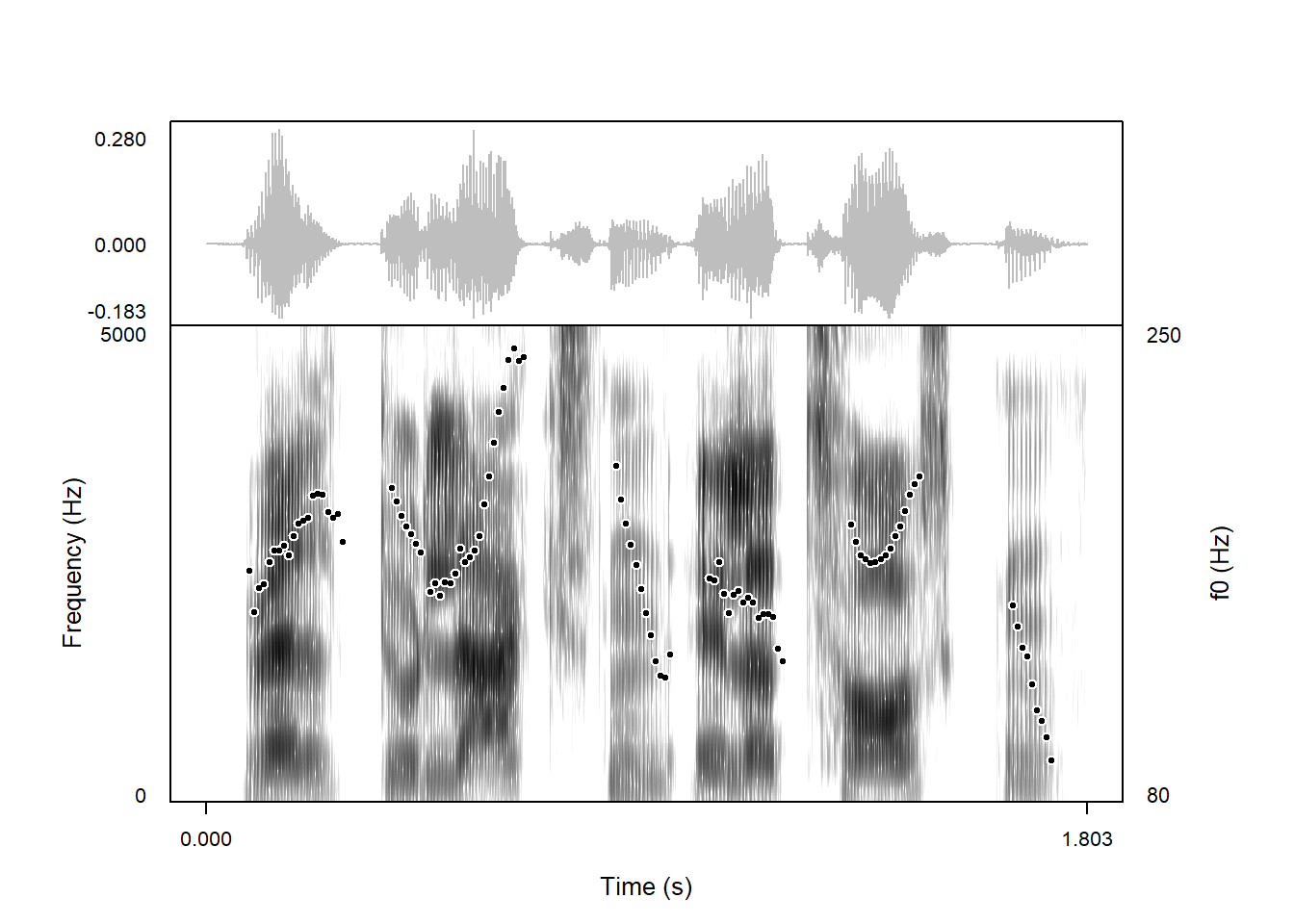
Notice that the y-axis label will match the color of the pitch trace.
When overlaying a pitch trace on a spectrogram, there is the added option of having a wider line with a separate background color, which helps the trace stand out more. For example, we may want the pitch trace in the above plot to have a light blue background color. In this case, we can pass a vector to pitch_color specifying first the main color, and then the background:
praatpicture('ex/ex.wav',
             frames = c('sound', 'spectrogram'),
             proportion = c(30,70),
             wave_color = 'grey',
             pitch_plotOnSpec = TRUE,
             pitch_color = c('blue', 'lightblue'),
             pitch_scale = 'log',
             pitch_freqRange = c(80,250),
             pitch_axisLabel = 'f0 (Hz)')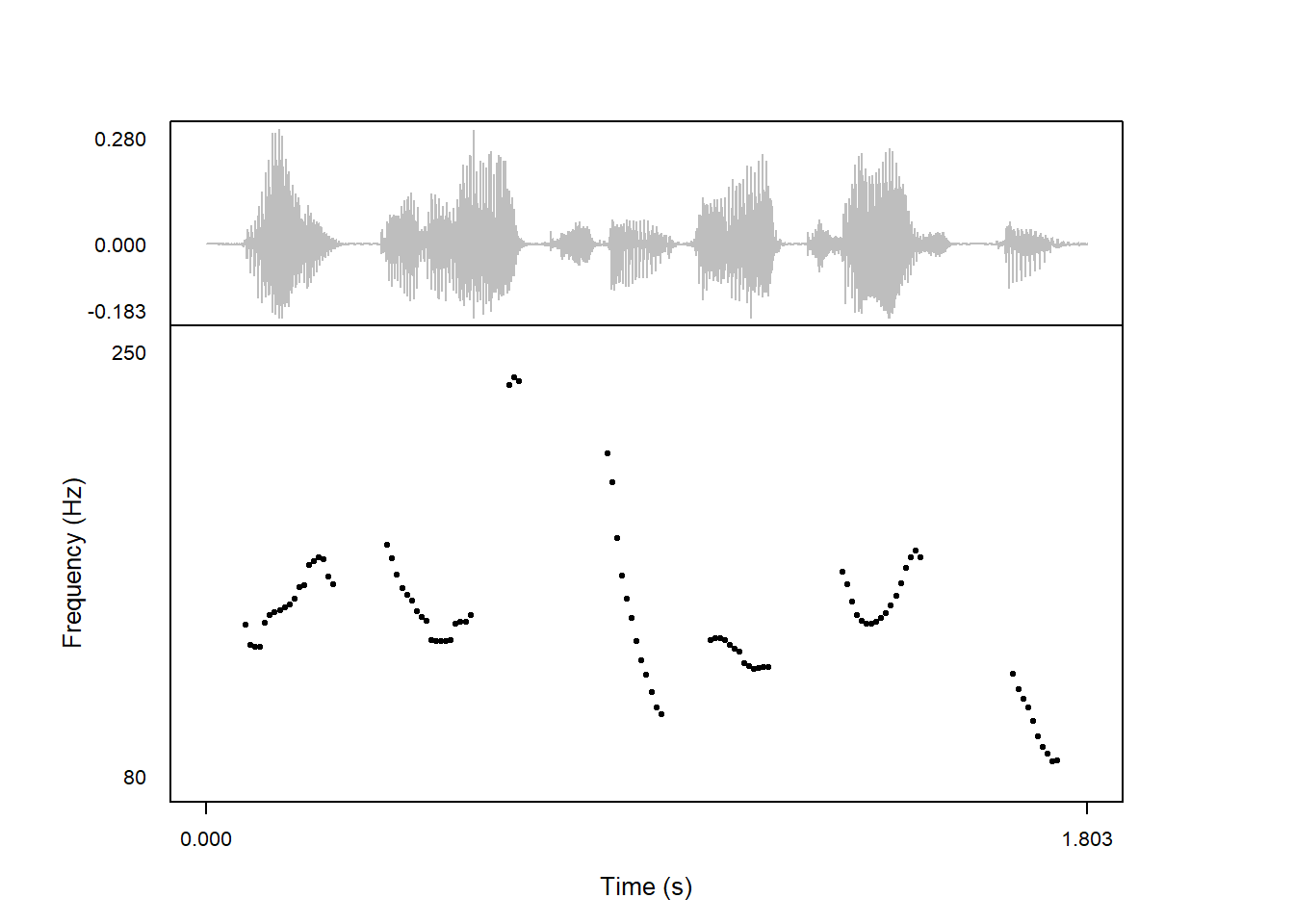
This will also work if pitch is ‘speckled’:
praatpicture('ex/ex.wav',
             frames = c('sound', 'spectrogram'),
             proportion = c(30,70),
             wave_color = 'grey',
             pitch_plotOnSpec = TRUE,
             pitch_plotType = 'speckle',
             pitch_color = c('black', 'white'),
             pitch_scale = 'log',
             pitch_freqRange = c(80,250),
             pitch_axisLabel = 'f0 (Hz)')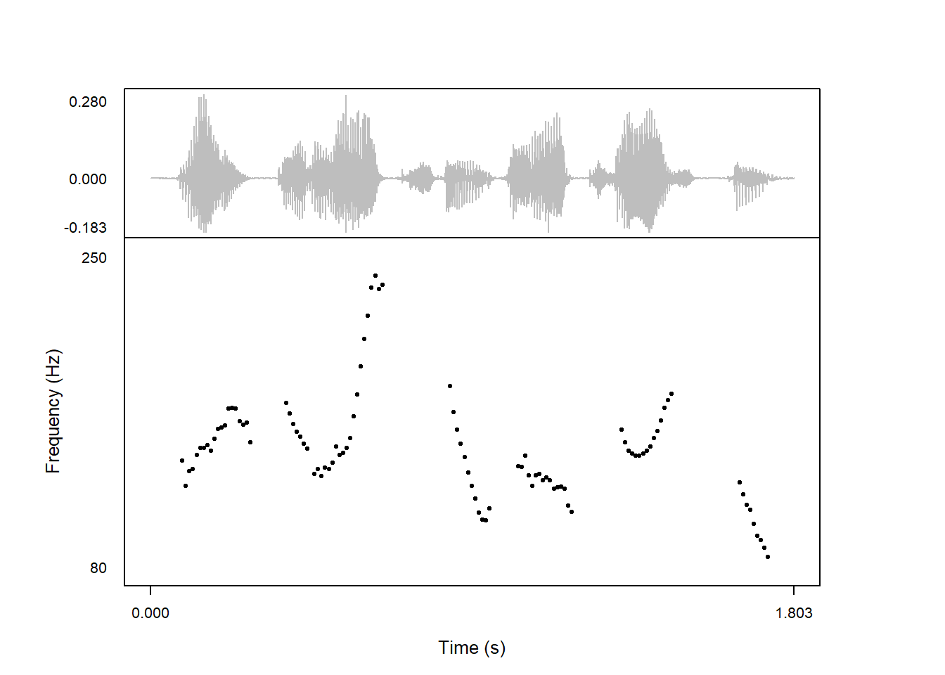
It’s also possible to overlay pitch on the waveform. This works much the same as overlaying pitch on the spectrogram, controlled with the pitch_plotOnWave argument.
praatpicture('ex/ex.wav',
             frames = c('sound', 'spectrogram'),
             proportion = c(50,50),
             wave_color = 'grey',
             pitch_plotOnWave = TRUE)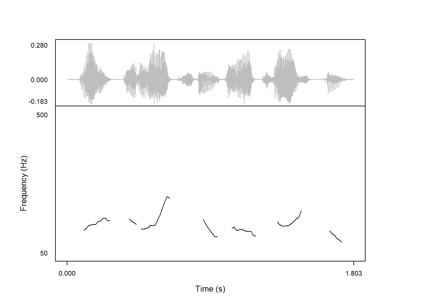
As above, all the default pitch plotting parameters also apply when plotting pitch on a waveform:
praatpicture('ex/ex.wav',
             frames = c('sound', 'spectrogram'),
             proportion = c(50,50),
             wave_color = 'grey',
             pitch_plotOnWave = TRUE,
             pitch_color = c('black','white'),
             pitch_scale = 'log',
             pitch_plotType = 'speckle',
             pitch_freqRange = c(80,250),
             pitch_axisLabel = 'f0 (Hz)')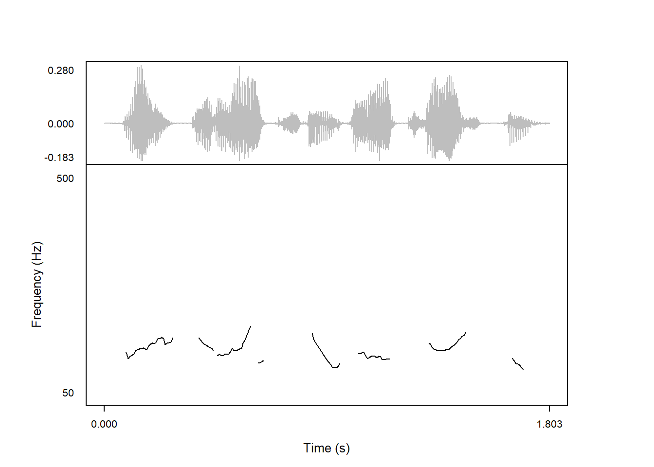
Pitch tracks are typically calculated on the fly in R using the ksvF0() function from the wrassp library, which is a convenient way to call functions from the C library libassp in R. ksvF0() implements the pitch detection method described by Schäfer-Vincent (1983).
There are several reasons why you may wish to use the signal processing tools from Praat instead. For example, Praat has a nice GUI allowing users to hand-edit the pitch contour, and if you’re writing about pitch and using Praat to generate the pitch contours, it could be important to show actual examples of the data you’re analyzing using the exact same parameter settings as you’re using for the analysis. And in all likelihood the pitch detection method used by Praat (described by Boersma 1993) is more accurate than the one implemented in ksvF0(). Luckily, it’s fairly straightforward to plot pitch contours in praatpicture that are calculated in Praat.
If you open and select a sound file in Praat, you can generate a pitch track by clicking the Analyse periodicity - button and selecting one of the To Pitch... options. Once you have done this, and you’ve potentially edited the pitch track according to your wishes, click the Save button and Save as text file..., and save the object using the same base name as your sound file and the .Pitch extension. If you have done this, praatpicture will automatically plot the values in the .PitchTier file instead of calculating pitch on the fly. Alternatively, you can click the Convert - button and select Down to PitchTier, and save this as a text file with the .PitchTier extension. It typically does not matter whether you plot a Pitch or PitchTier object, but you may see some unwanted interpolation if you plot longer PitchTier objects with pitch_plotType = 'speckle'.
As an example, this is a copy of the file that we’ve used throughout this section, which has a corresponding .PitchTier file (i.e., pitch is generated in Praat):
praatpicture('ex/ex_praatsp.wav',
             frames = c('sound', 'pitch'),
             proportion = c(30,70),
             wave_color = 'grey',
             pitch_plotType = 'speckle',
             pitch_freqRange = c(80,250))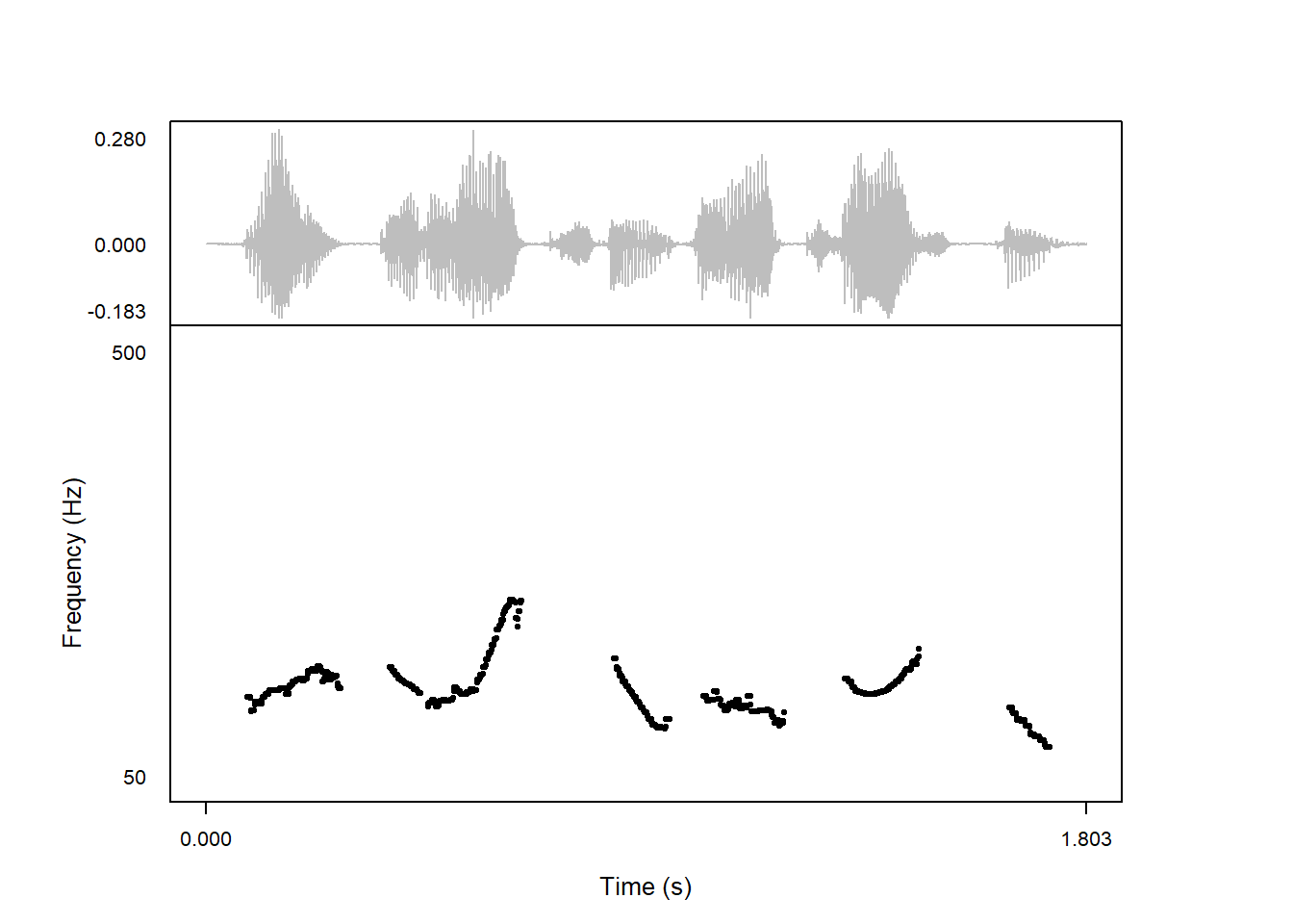
And this is that same snippet with pitch generated in R on the fly:
praatpicture('ex/ex.wav',
             frames = c('sound', 'pitch'),
             proportion = c(30,70),
             wave_color = 'grey',
             pitch_plotType = 'speckle',
             pitch_freqRange = c(80,250))
Reasonably similar results, but the ksvF0() contour is sometimes a bit more jagged, and it detects a rise that Praat does not find!
Note that the signal processing options introduced below are only used when calculating pitch on the fly in R. If pitch is plotted from a .PitchTier file, they are ignored – in this case, you need to set your own signal processing parameters in Praat!
As we will see in Section 15.3, any method can in principle be used for calculating the plotted pitch tracks as long as the results are formatted in a particular way.
The parameters used to predict pitch do not use ksvF0() defaults, but are rather set to emulate Praat as closely as possible. Some of these can’t be changed (using Gaussian-shaped KAISER2_0 windows), but some can! You’ll find that some of the settings which can be toggled in Praat are not necessarily available in praatpicture, either because ksvF0() doesn’t allow you to change them, or because these settings are specific to the pitch tracking algorihtm(s) used in Praat.
The lowest and highest pitch to look for is controlled with the pitch_floor and pitch_ceiling parameters. By default, praatpicture searches between 75–600 Hz, which is in most cases fine for plotting, but is worth limiting if you see octave jumps in the resulting plots.
Increasing the range to 50–800 Hz does not change much, but provides a slightly smoother contour (probably because the measurement interval depends on these settings; see below).
praatpicture('ex/ex.wav',
             frames = c('sound', 'pitch'),
             proportion = c(30,70),
             wave_color = 'grey',
             pitch_floor = 50,
             pitch_ceiling = 800)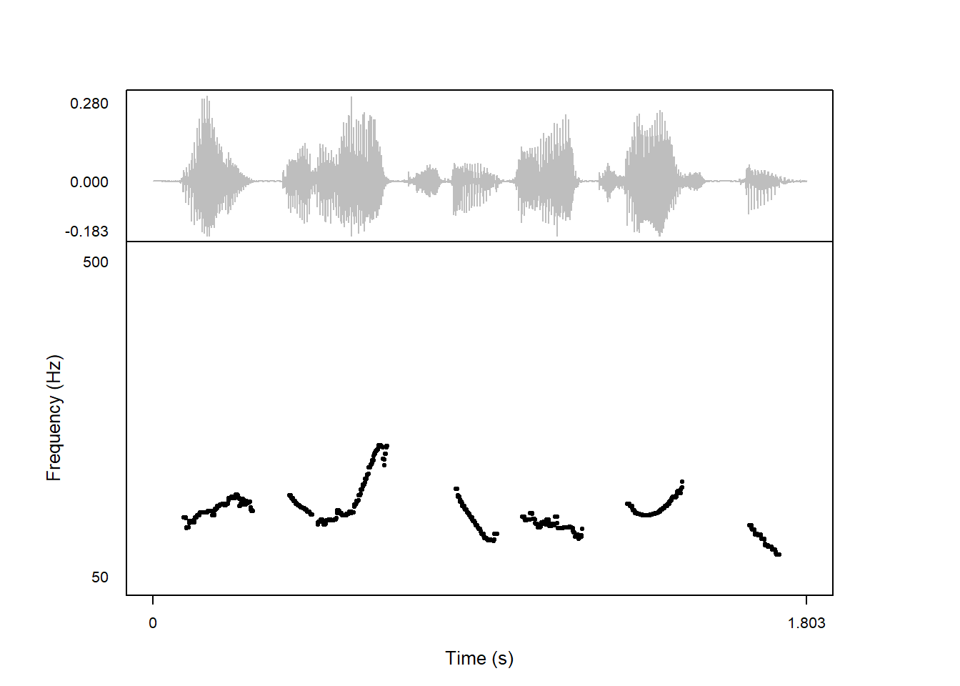
We’ll mostly see a change if we drastically reduce the range. Here I’ve set it to 100–200 Hz, i.e. a ceiling well below the higher range of this speaker. Here you’ll see that higher frequencies are missing:
praatpicture('ex/ex.wav',
             frames = c('sound', 'pitch'),
             proportion = c(30,70),
             wave_color = 'grey',
             pitch_floor = 100,
             pitch_ceiling = 200)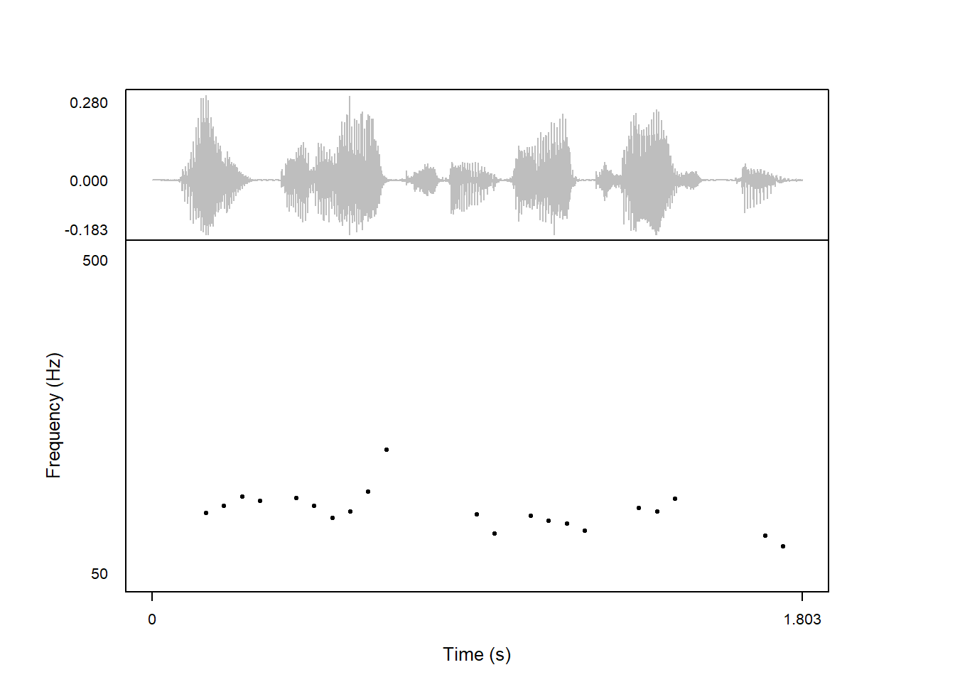
The intervals at which to measure pitch is controlled with the pitch_timeStep parameter. The default here is to calculate the measurement interval dynamically based on the pitch_floor, such that it is \(\frac{3}{4}\) pitch_floor, which with the default floor of 75 Hz amounts to 0.01, i.e. every 10 ms. But users can also specify a number (in ms). Here we take a lot more measures, once per ms:
praatpicture('ex/ex.wav',
             frames = c('sound', 'pitch'),
             proportion = c(30,70),
             wave_color = 'grey',
             pitch_plotType = 'speckle',
             pitch_timeStep = 0.001)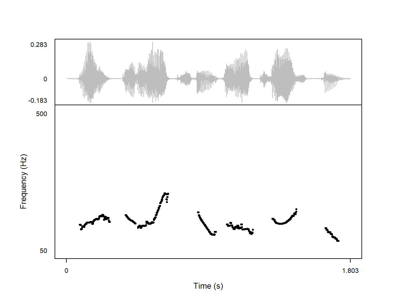
And this is what it looks like with fewer measures, once every 50 ms:
praatpicture('ex/ex.wav',
             frames = c('sound', 'pitch'),
             proportion = c(30,70),
             wave_color = 'grey',
             pitch_plotType = 'speckle',
             pitch_timeStep = 0.05)