praatpicture('ex/fmt.wav',
             frames = c('sound', 'formant'),
             proportion = c(30,70),
             wave_color = 'grey')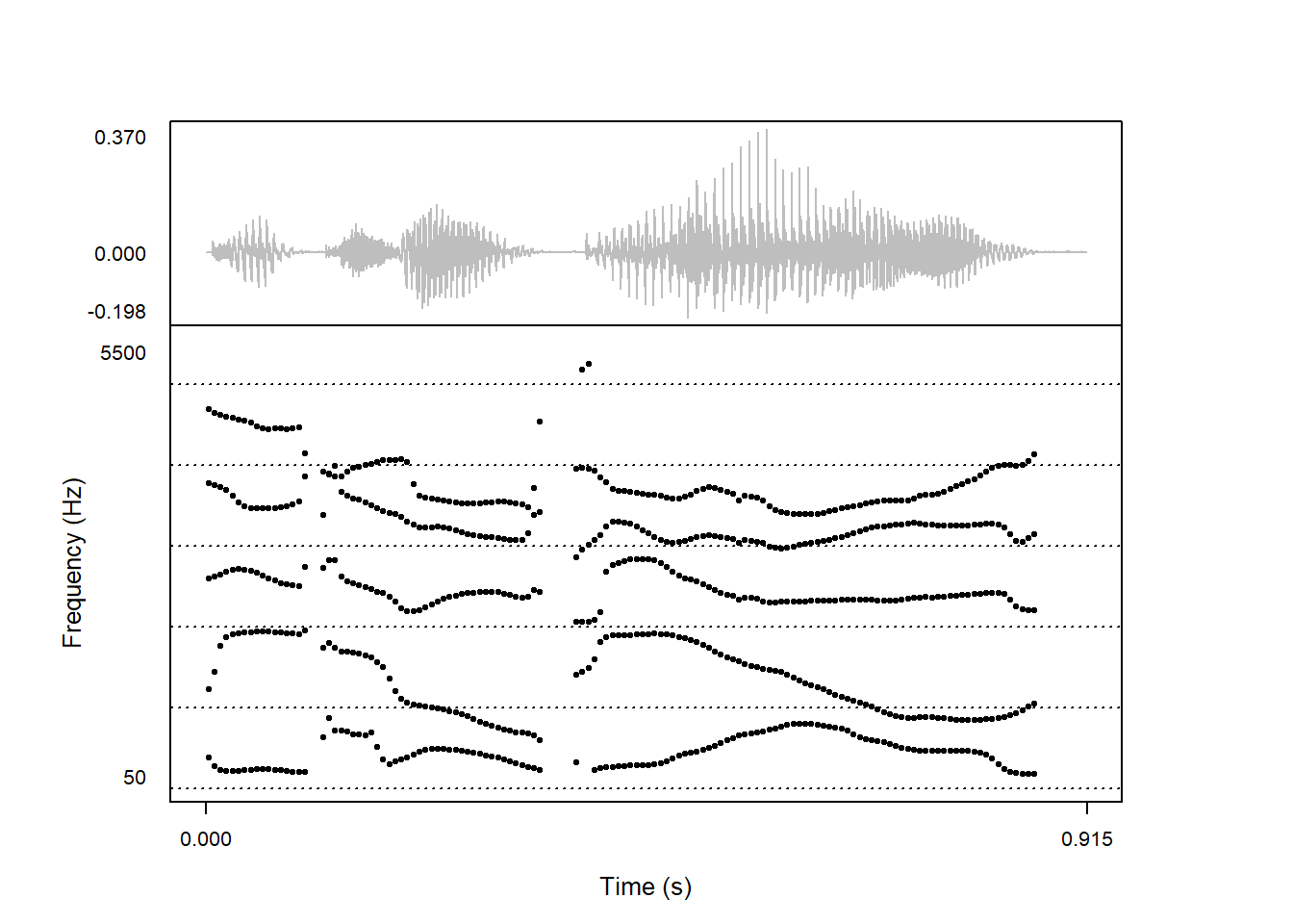
The formant tracks plotted by praatpicture by default look similar to those produced by Praat, but users have a lot of options regarding both the general appearance of formant tracks and the underlying signal processing, or to capitalize on the signal processing provided by Praat (see Section 7.2). We’ll cover those options here.
When plotting formants in Praat, formant tracks are either ‘drawn’ or ‘speckled’. The default is ‘speckled’, i.e. point plots:
praatpicture('ex/fmt.wav',
frames = c('sound', 'formant'),
proportion = c(30,70),
wave_color = 'grey')
This can be controlled with the formant_plotType argument. A ‘drawn’ plot will produce a line plot:
praatpicture('ex/fmt.wav',
             frames = c('sound', 'formant'),
             proportion = c(30,70),
             wave_color = 'grey',
             formant_plotType = 'draw')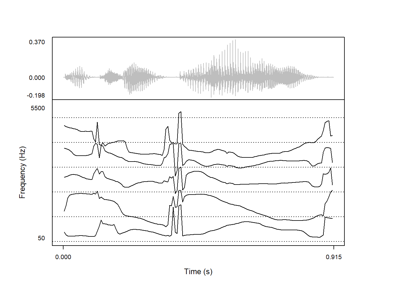
This will look really erratic for sequences of speech where there aren’t supposed to be any vowels, but looks alright when e.g. plotting a diphthong, as we can see if we plot just a portion of this sound:
praatpicture('ex/fmt.wav',
             start = 0.4, end = 0.85,
             frames = c('sound', 'formant'),
             proportion = c(30,70),
             wave_color = 'grey',
             formant_plotType = 'draw')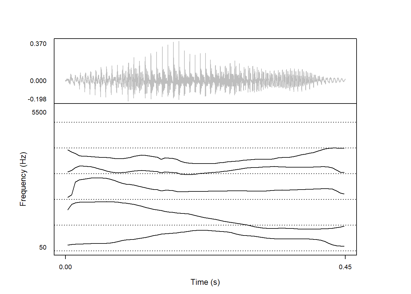
If you want to draw formant contours with thicker, you can set the drawSize argument larger than 1 (which will also affect other drawn derived signals, i.e. pitch or intensity).
praatpicture('ex/fmt.wav',
             start = 0.4, end = 0.85,
             frames = c('sound', 'formant'),
             proportion = c(30,70),
             wave_color = 'grey',
             formant_plotType = 'draw',
             drawSize = 3)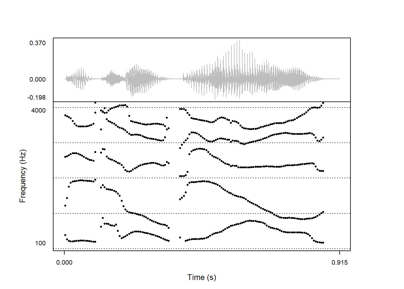
The speckleSize argument works similarly if you want larger points in a speckled plot.
praatpicture('ex/fmt.wav',
             frames = c('sound', 'formant'),
             proportion = c(30,70),
             wave_color = 'grey',
             speckleSize = 2)
The formant_number argument controls how many formants to show. Here we plot only the first three formants:
praatpicture('ex/fmt.wav',
             frames = c('sound', 'formant'),
             proportion = c(30,70),
             wave_color = 'grey',
             formant_number = 3)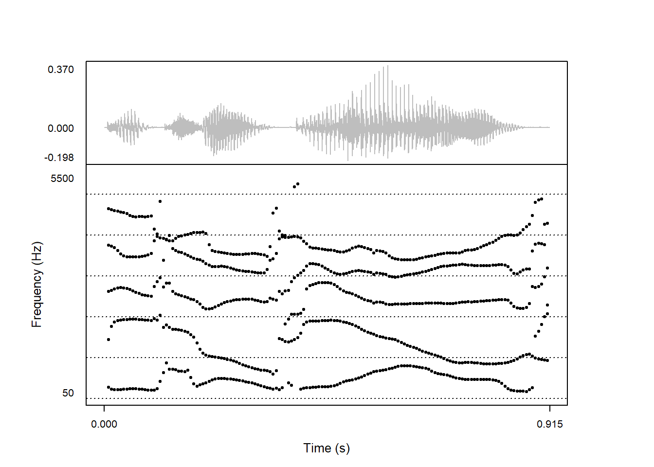
Note that this is not the same as only estimating three formants, which is controlled with the formant_maxN argument as shown below. Changing formant_maxN will change the signal processing, while formant_number only controls how many formants are shown in the plot. You will get an error if formant_number is higher than formant_maxN.
The default frequency range for formant plots shows between 50–5500 Hz. This is rather broad for most purposes. Frequency range can be controlled with the formant_freqRange argument. Here, a frequency range between 100–4000 Hz is probably more suitable:
praatpicture('ex/fmt.wav',
             frames = c('sound', 'formant'),
             proportion = c(30,70),
             wave_color = 'grey',
             formant_freqRange = c(100,4000))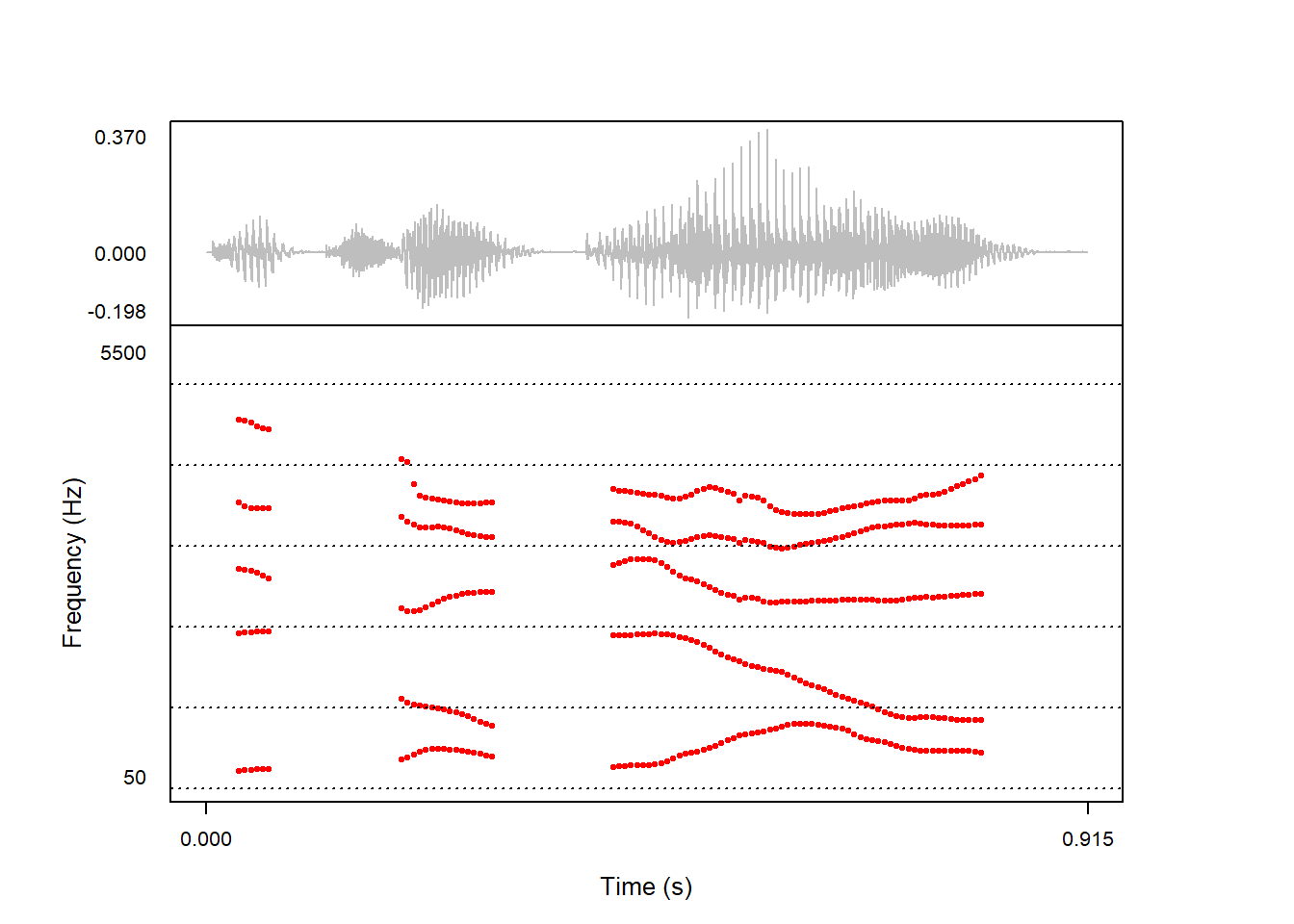
The dynamic range of the formant track is set to 30 dB by default, meaning that only formant measures taken from windows of the sound file with energy within the highest 30 dB in the plotted sound snippet are rendered; at least in ‘speckled’ plots, all other measures are ignored. This can be controlled with the formant_dynamicRange argument.
In the plots above, it is clear that formants are sometimes included from portions of speech that aren’t actually vowels. If we reduce formant_dynamicRange, there’s a higher chance that formants are only plotted from vowels. Here shown with a dynamic range of just 8 dB:
praatpicture('ex/fmt.wav',
             frames = c('sound', 'formant'),
             proportion = c(30,70),
             wave_color = 'grey',
             formant_dynamicRange = 8)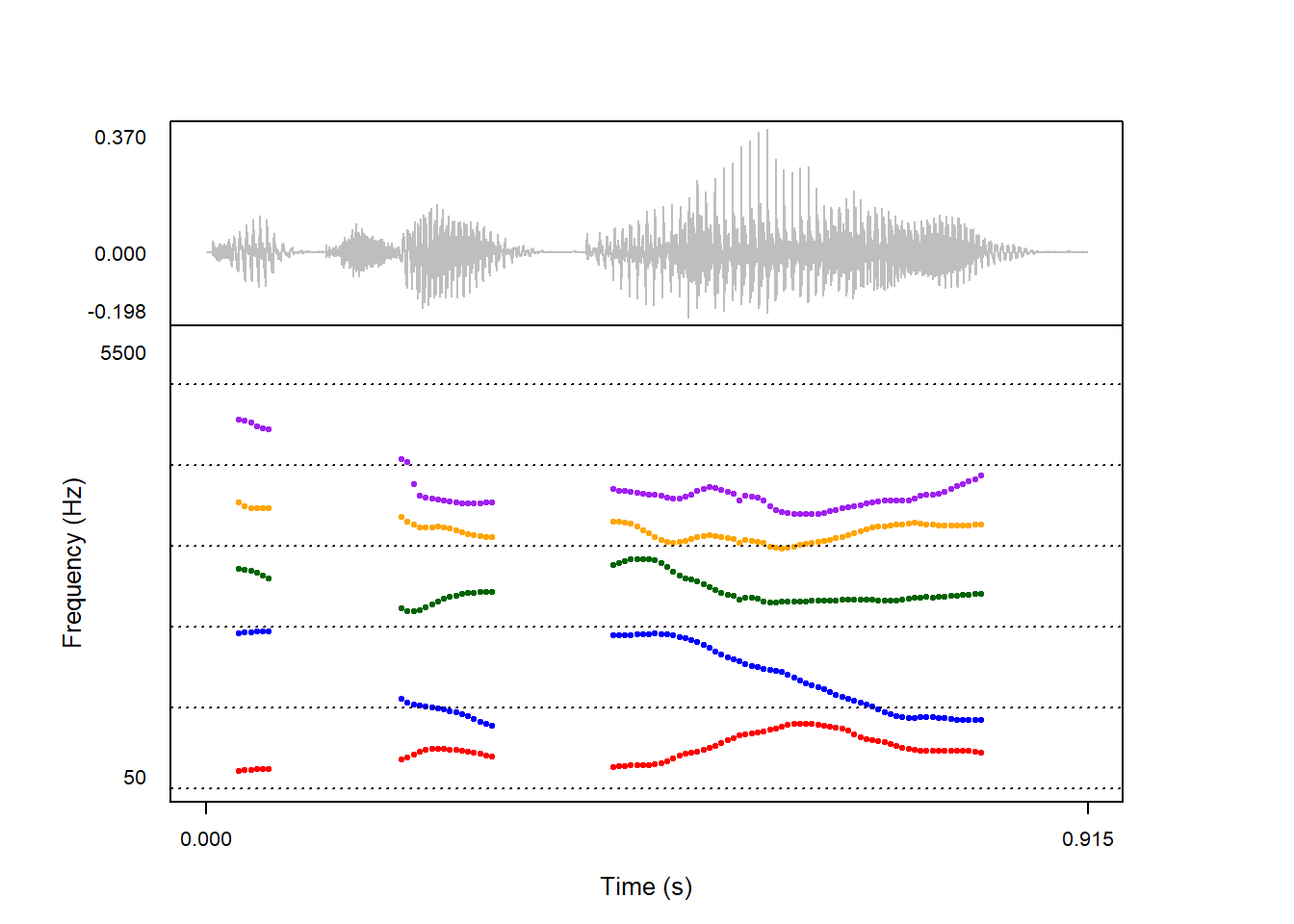
If we increase the dynamic range, we’ll see that formants are being predicted all over the place. Here with a dynamic range of 50 dB:
praatpicture('ex/fmt.wav',
             frames = c('sound', 'formant'),
             proportion = c(30,70),
             wave_color = 'grey',
             formant_dynamicRange = 50)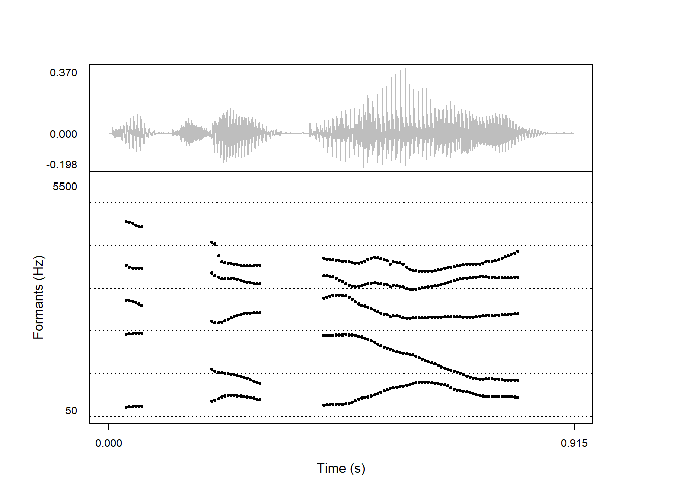
The color of the formant tracks can be controlled with the formant_color argument. Here are formants plotted in red:
praatpicture('ex/fmt.wav',
             frames = c('sound', 'formant'),
             proportion = c(30,70),
             wave_color = 'grey',
             formant_dynamicRange = 8,
             formant_color = 'red')
It is possible to use different colors for different formant values, by passing a vector to formant_color with as many colors as the number of formants being plotted. This can help differentiate the different formants in more complex plots:
praatpicture('ex/fmt.wav',
             frames = c('sound', 'formant'),
             proportion = c(30,70),
             wave_color = 'grey',
             formant_dynamicRange = 8,
             formant_color = c('red', 'blue', 'darkgreen', 'orange', 'purple'))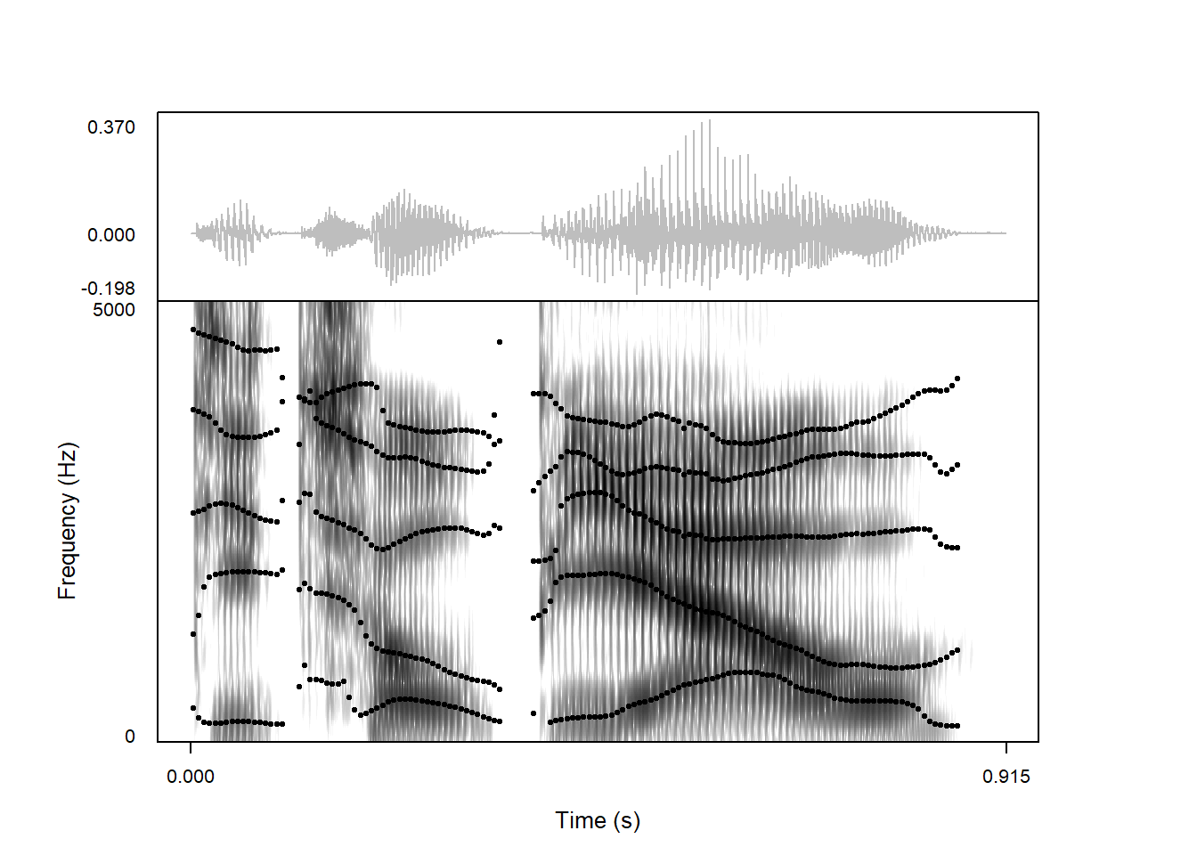
Some fancier coloring options are available when formants are overlaid on spectrograms; more on that in Section 7.1.8.
Users can specify their own axis labels, using the formant_axisLabel argument. For example, we might want to specify that they are formants:
praatpicture('ex/fmt.wav',
             frames = c('sound', 'formant'),
             proportion = c(30,70),
             wave_color = 'grey',
             formant_dynamicRange = 8,
             formant_axisLabel = 'Formants (Hz)')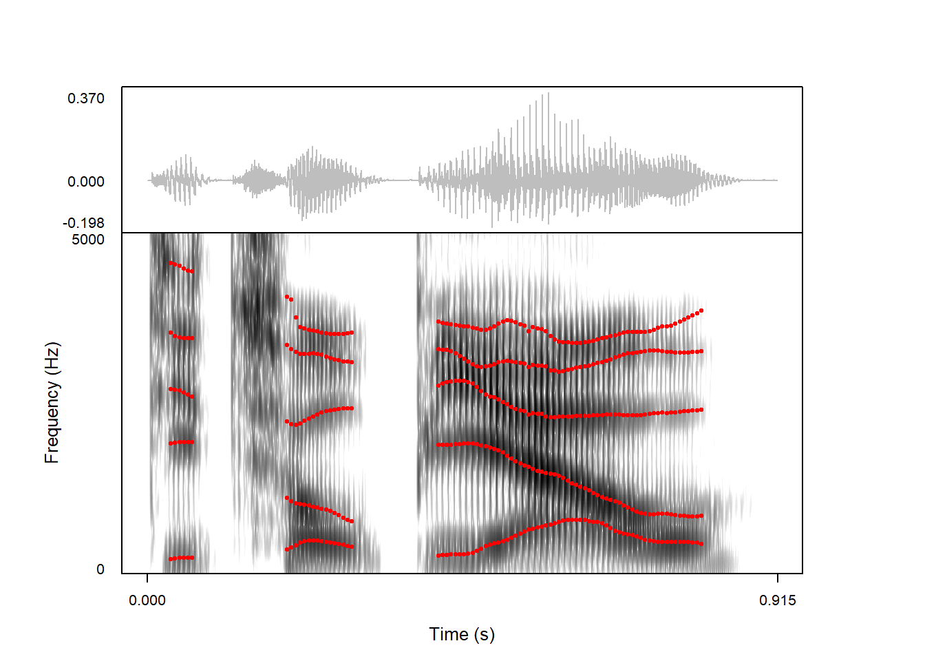
Following the Praat defaults for formant plotting, horizontal dotted lines are shown in formant plots at multiples of 1000 Hz. This is controlled with the general draw_lines argument, and you can override the default dotted lines by setting draw_lines to NULL:
praatpicture('ex/fmt.wav',
             frames = c('sound', 'formant'),
             proportion = c(30,70),
             wave_color = 'grey',
             formant_dynamicRange = 8,
             draw_lines = NULL)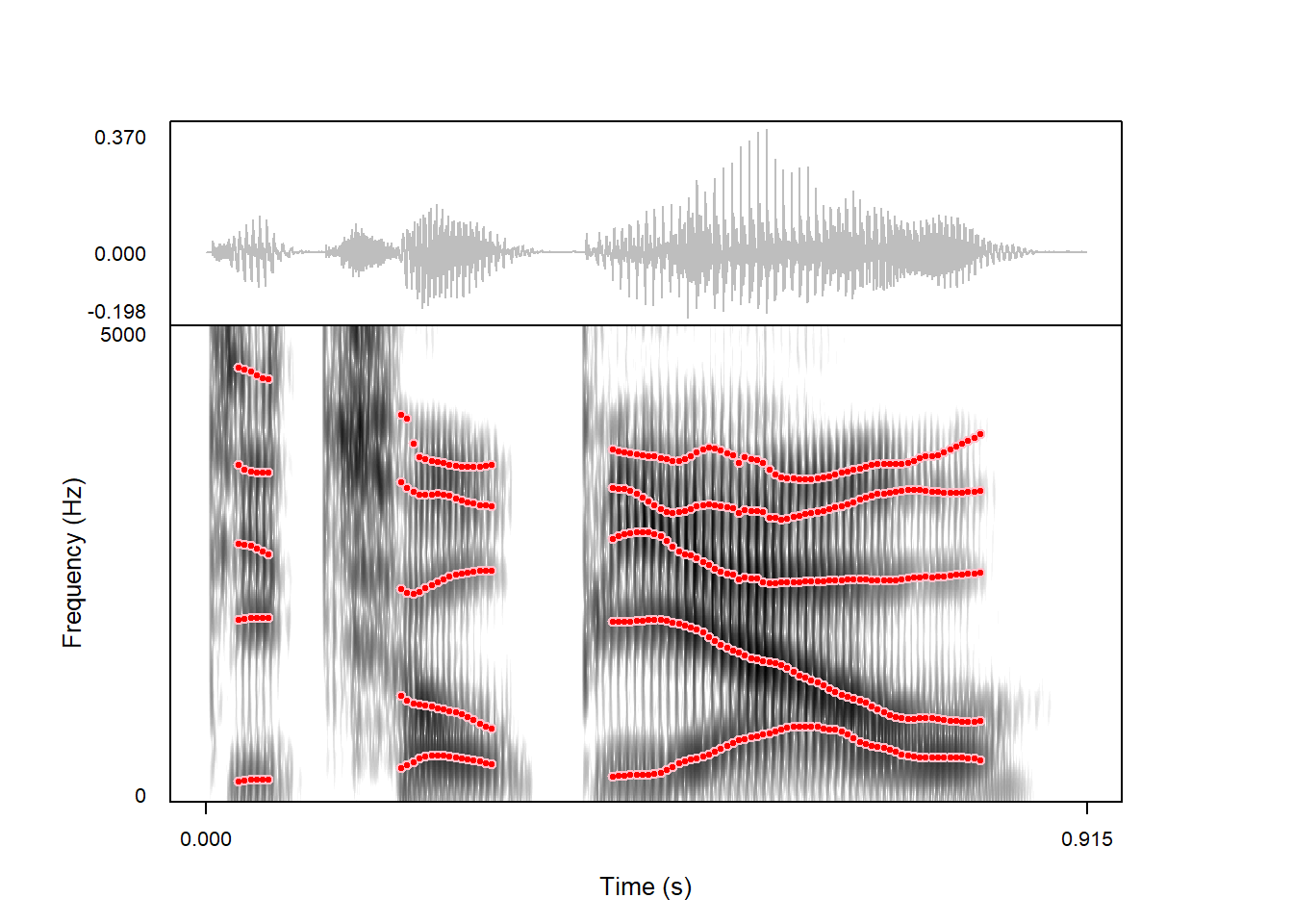
More on draw_lines in Section 9.4.
Instead of drawing formants in their own frame, it is also possible to overlay formants on a spectrogram. In this case, formant should not be specified as one of the frames; this is instead controlled with the Boolean formant_plotOnSpec argument.
praatpicture('ex/fmt.wav',
             frames = c('sound', 'spectrogram'),
             proportion = c(30,70),
             wave_color = 'grey',
             formant_plotOnSpec = TRUE)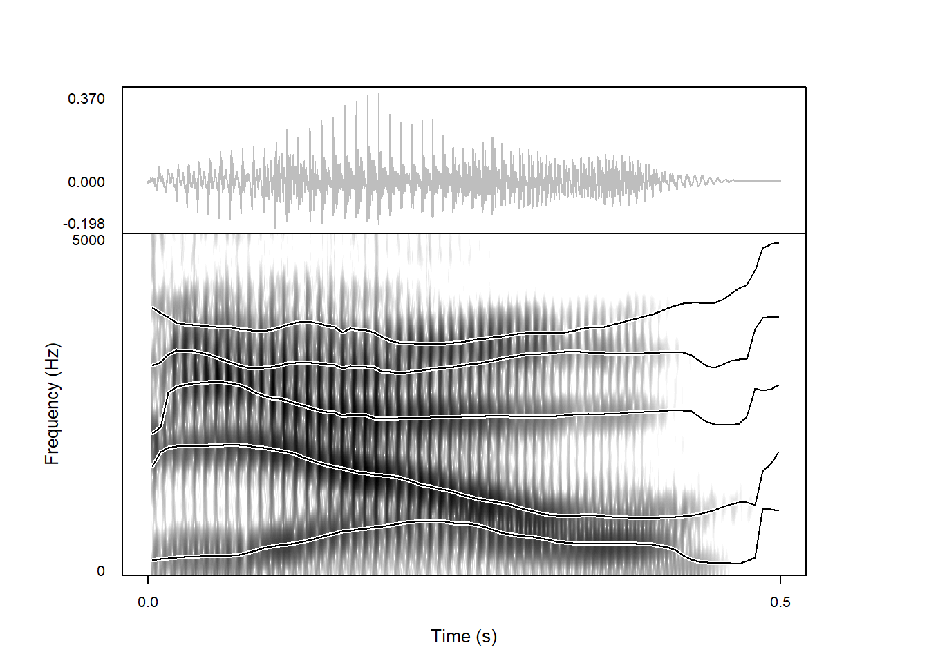
The other arguments controlling formant appearance (and signal processing) also work when overlaying formants on the spectrogram. For example, we clearly see above that a dynamic range of 30 dB is too high for this file, and that 8 dB is more suitable. Also, formants overlaid on a spectrogram stand out much more if they are not plotted in black.
praatpicture('ex/fmt.wav',
             frames = c('sound', 'spectrogram'),
             proportion = c(30,70),
             wave_color = 'grey',
             formant_plotOnSpec = TRUE,
             formant_dynamicRange = 8,
             formant_color = 'red')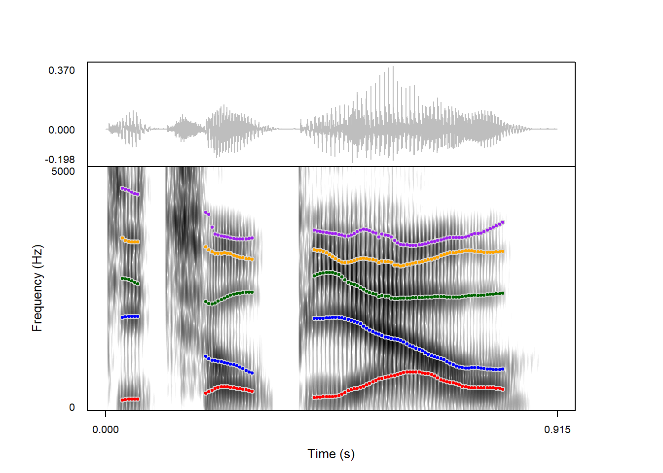
When overlaying formants on a spectrogram, there is the added option of having a wider point with a separate background color, which helps the trace stand out more. For example, we may want the formants in the above plot to have a pink background color. In this case, we can pass a vector to pitch_color specifying first the main color, and then the background:
praatpicture('ex/fmt.wav',
             frames = c('sound', 'spectrogram'),
             proportion = c(30,70),
             wave_color = 'grey',
             formant_plotOnSpec = TRUE,
             formant_dynamicRange = 8,
             formant_color = c('red', 'pink'))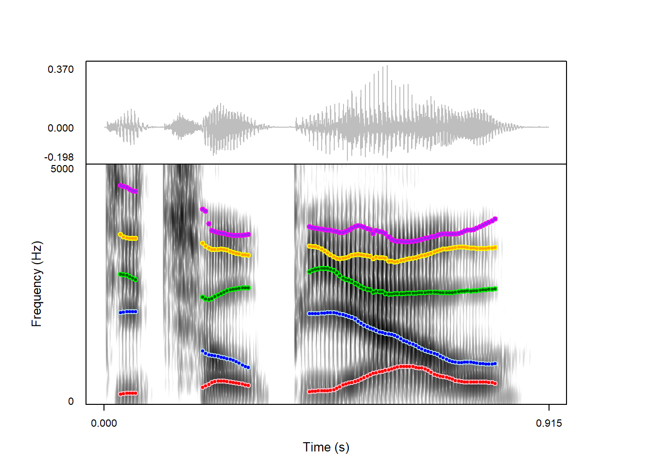
This will also work when producing a ‘drawn’ plot:
praatpicture('ex/fmt.wav',
             start = 0.4, end = 0.9,
             frames = c('sound', 'spectrogram'),
             proportion = c(30,70),
             wave_color = 'grey',
             formant_plotOnSpec = TRUE,
             formant_plotType = 'draw',
             formant_color = c('black', 'white'))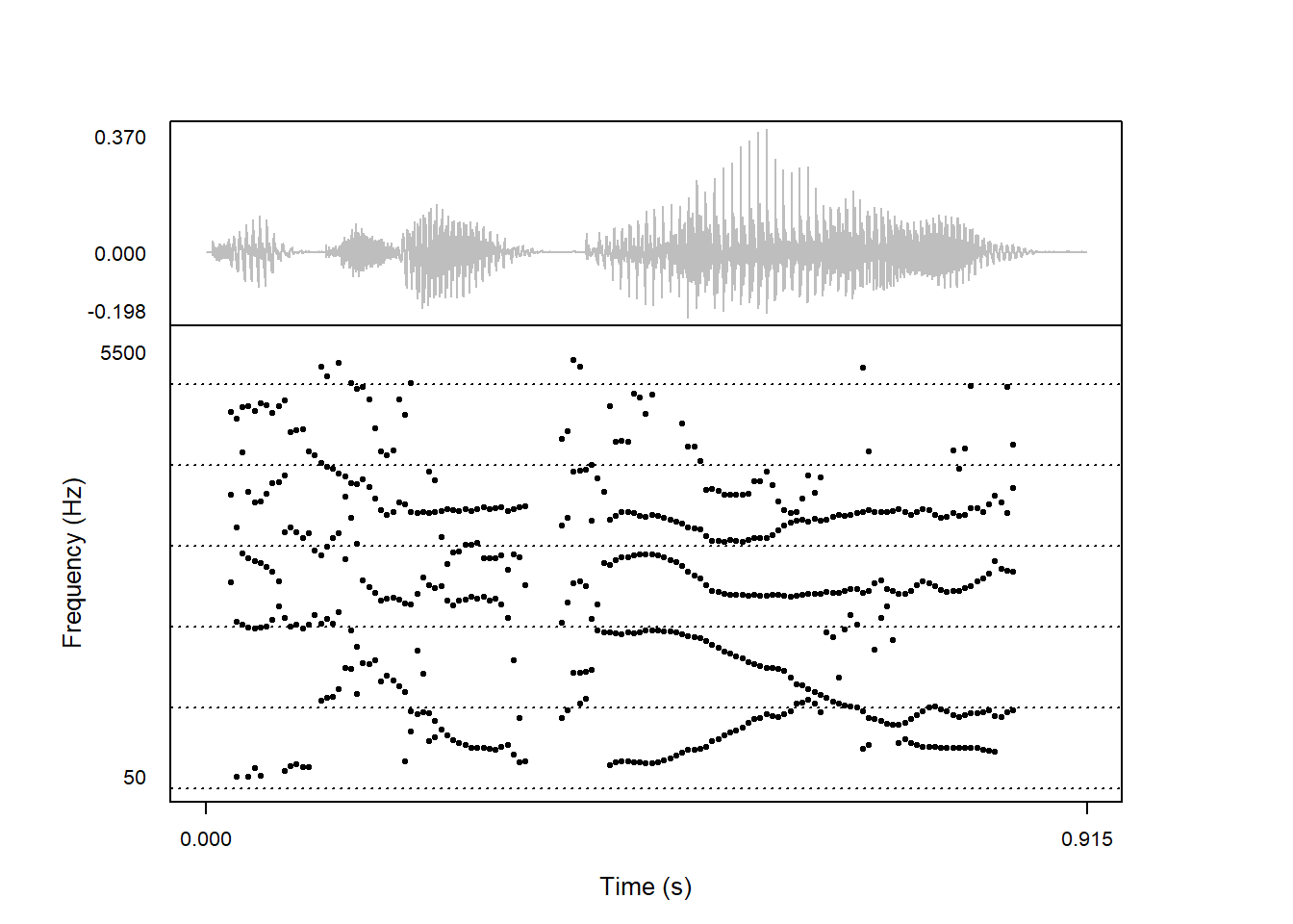
If you’re using different colors for different formants, you can pass a vector with one more color than the number of formants being plotted, and then the last one will be used for the background. Here with a light grey background:
praatpicture('ex/fmt.wav',
             frames = c('sound', 'spectrogram'),
             proportion = c(30,70),
             wave_color = 'grey',
             formant_plotOnSpec = TRUE,
             formant_dynamicRange = 8,
             formant_color = c('red', 'blue', 'darkgreen', 'orange', 'purple',
                               'lightgrey'))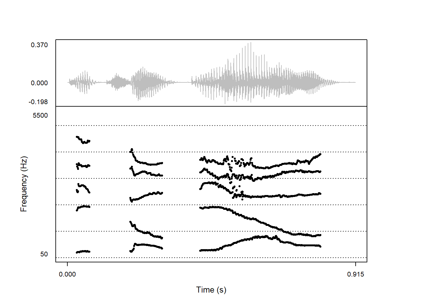
You can also pass a vector with twice as many colors as the formants being plotted. In this case, the last half will be used for background colors:
praatpicture('ex/fmt.wav',
             frames = c('sound', 'spectrogram'),
             proportion = c(30,70),
             wave_color = 'grey',
             formant_plotOnSpec = TRUE,
             formant_dynamicRange = 8,
             formant_color = c('red', 'blue', 'darkgreen', 'orange', 'purple',
                               'pink', 'lightblue', 'green', 'yellow',
                               'magenta'))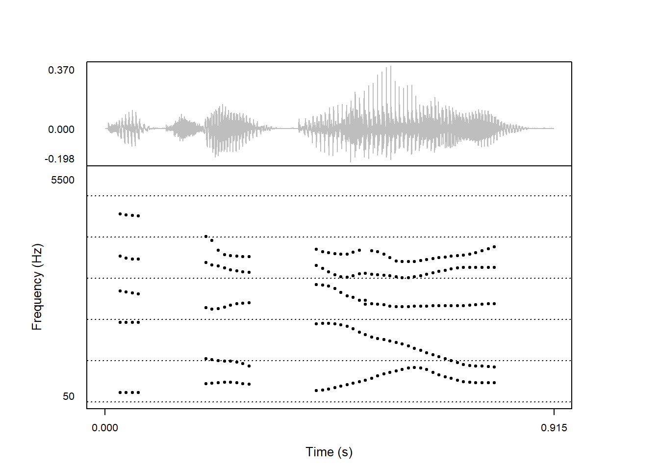
As shown in Chapter 5, a few other frequency scales are available in praatpicture() in addition to linear Hertz. Formant overlays also works with ERB and Mel-scaled spectrograms, as shown here for a Mel-scaled spectrogram:
praatpicture('ex/fmt.wav',
             frames = c('sound', 'spectrogram'),
             proportion = c(30,70),
             wave_color = 'grey',
             formant_plotOnSpec = TRUE,
             formant_dynamicRange = 8,
             formant_color = c('red', 'pink'),
             spec_color = c('white', 'blue'),
             spec_scale = 'mel',
             spec_freqRange = c(0,3500))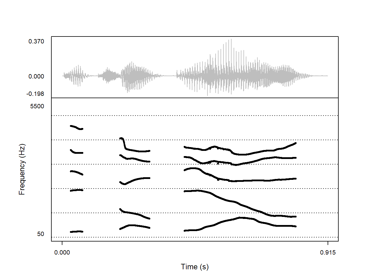
Formants are typically calculated on the fly in R using the forest() function from the wrassp library, which is a convenient way to call functions from the C library libassp in R. forest() uses the split-Levinson algorithm to detect formants as implemented by Willems (1987).
There are several reasons why you may wish to use the signal processing tools from Praat instead. For example, if you’re writing about formants and using Praat to calculate the formants, it could be important to show actual examples of the data you’re analyzing using the exact same parameter settings as you’re using for the analysis. And in all likelihood the Burg algorithm that Praat uses for formant detection method is more accurate than the one implemented in forest(), as the Praat documentation specifically alludes to. Luckily, it’s fairly straightforward to plot formants in praatpicture that are calculated in Praat.
If you open and select a sound file in Praat, you can generate a formant track by clicking the Analyse spectrum - button and selecting one of the To Formant... options. Once you have done this, and you’ve potentially edited the formant track according to your wishes, click the Save button and select Save as text file..., and save the object using the same base name as your sound file and the .Formant extension. If you have done this, praatpicture will automatically plot the values in the .Formant file instead of calculating formants on the fly.
As an example, this is a copy of the file that we’ve used throughout this section, which has a corresponding .Formant file (i.e., formants are calculated in Praat):
praatpicture('ex/fmt_praatsp.wav',
             frames = c('sound', 'formant'),
             proportion = c(30,70),
             wave_color = 'grey',
             formant_dynamicRange = 30)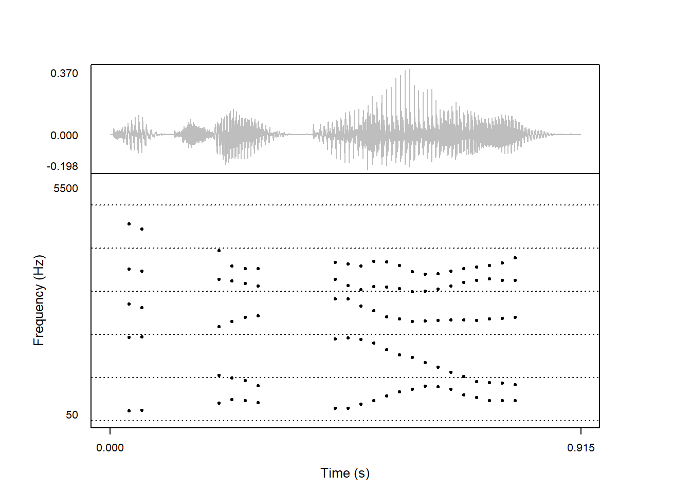
In this particular case, the Praat-calculated formant tracks are in fact highly erratic, much more so than the forest()-calculated formants.
Note that the signal processing options introduced below are only used when calculating formants on the fly in R. If formants are plotted from a .Formant file, they are ignored – in this case, you need to set your own signal processing parameters in Praat!
As we will see in Section 15.3, any method can in principle be used for calculating the plotted formants as long as the results are formatted in a particular way.
The parameters used to predict formants do not use forest() defaults, but are rather set to emulate Praat as closely as possible. Some of these can’t be changed (using Gaussian-shaped KAISER2_0 windows), but some can! You’ll find that some of the settings which can be toggled in Praat are not necessarily available in praatpicture (unfortunately including a formant ceiling parameter setting a maximum search range), either because forest() doesn’t allow you to change them, or because these settings are specific to the formant tracking algorihtm(s) used in Praat.
Users can control the effective length of windows in which to search for formants with the formant_windowLength argument. The default is 25 ms. If we reduce the size of this window to e.g. 5 ms, it does not clearly result in worse predictions for the lower formants, but the higher formants are clearly more poorly tracked.
praatpicture('ex/fmt.wav',
             frames = c('sound', 'formant'),
             proportion = c(30,70),
             wave_color = 'grey',
             formant_dynamicRange = 8,
             formant_windowLength = 0.005)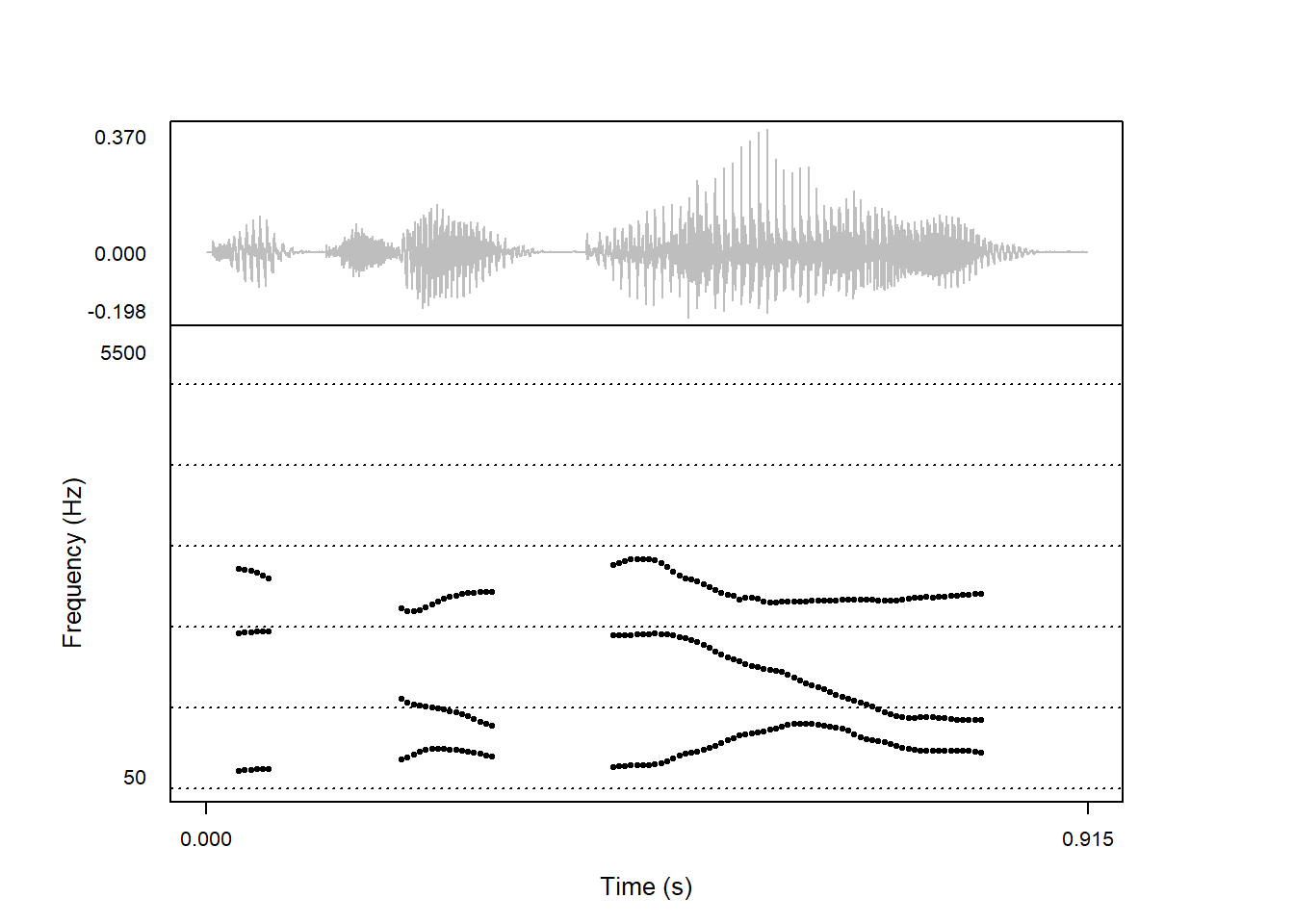
The algorithm seems less sensitive to increasing the window length, although this does increase the processing time and probably does not have many clear benefits. Here with a window length of 50 ms:
praatpicture('ex/fmt.wav',
             frames = c('sound', 'formant'),
             proportion = c(30,70),
             wave_color = 'grey',
             formant_dynamicRange = 8,
             formant_windowLength = 0.05)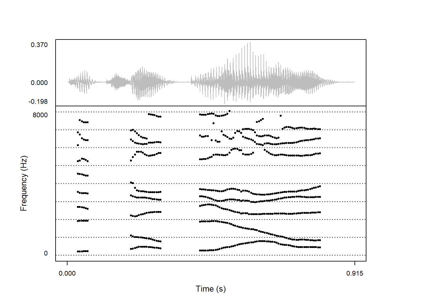
The intervals a which to measure formants is controlled with the formant_timeStep parameter. The default here is to calculate the measurement interval dynamically calculated based on the formant_windowLength, such that it is \(\frac{1}{4}\) formant_windowLength, which with the default window length of 25 ms amounts to 0.00625, i.e. every 6.25 ms. But users can also specify a number (in ms). Here we take a lot more measures, once per ms:
praatpicture('ex/fmt.wav',
             frames = c('sound', 'formant'),
             proportion = c(30,70),
             wave_color = 'grey',
             formant_dynamicRange = 8,
             formant_timeStep = 0.001)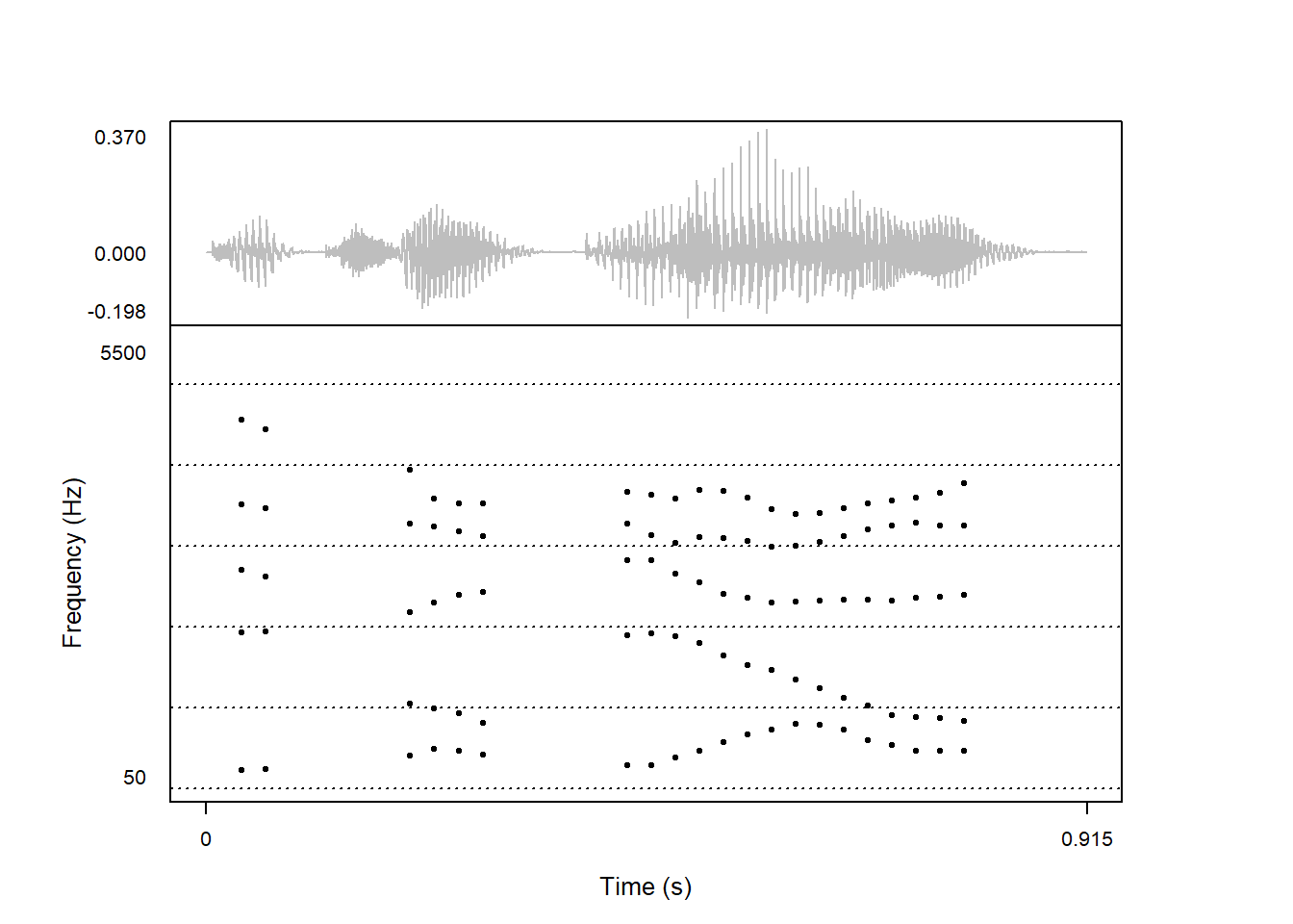
And this is what it looks like with fewer measures, once every 25 ms:
praatpicture('ex/fmt.wav',
             frames = c('sound', 'formant'),
             proportion = c(30,70),
             wave_color = 'grey',
             formant_dynamicRange = 8,
             formant_timeStep = 0.025)
You might think that the estimated number of formants is primarily an appearance parameter, but in fact the number of formants estimated can affect the overall results a fair bit. The number of formants to estimate is controlled with the formant_maxN parameter, which is by default set to 5. For this particular sound file, reducing the number of formants to 3 does not change the estimation of those 3 formants much:
praatpicture('ex/fmt.wav',
             frames = c('sound', 'formant'),
             proportion = c(30,70),
             wave_color = 'grey',
             formant_dynamicRange = 8,
             formant_maxN = 3)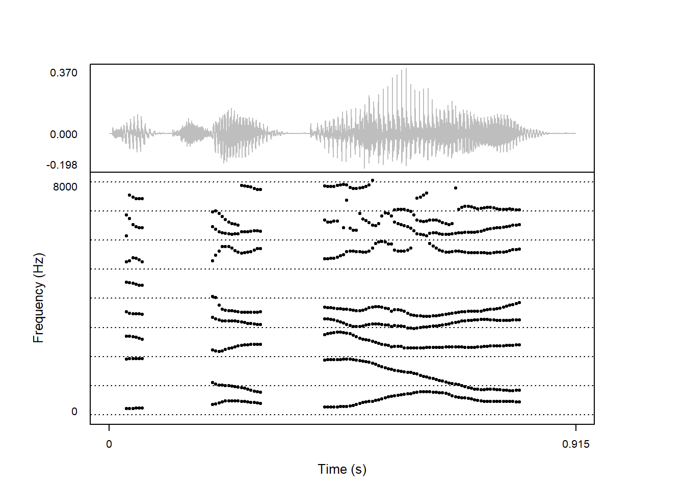
We could also set the number higher. Here, we estimate 8 formants:
praatpicture('ex/fmt.wav',
             frames = c('sound', 'formant'),
             proportion = c(30,70),
             wave_color = 'grey',
             formant_dynamicRange = 8,
             formant_freqRange = c(0,8000),
             formant_maxN = 8)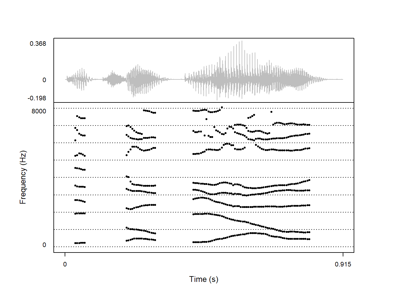
This could be useful, but you’ll note that the algorithm is less effective for higher formants.