praatpicture('ex/ex.wav',
             frames = c('sound', 'intensity'),
             proportion = c(30,70),
             wave_color = 'grey',
             intensity_range = c(0,80))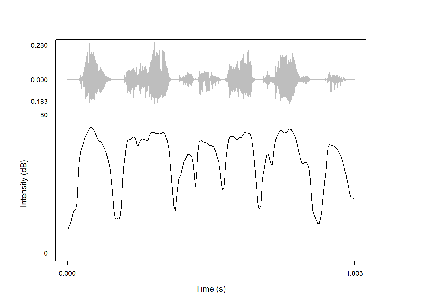
The intensity contours plotted by praatpicture by default look similar to those produced by Praat, but users have several options regarding both the general appearance of intensity contours and the underlying signal processing, or to capitalize on the signal processing provided by Praat (see Section 8.2). We’ll cover those options here.
By default, the amplitude range for intensity plots is dynamically determined to show the entire contour. The amplitude range can be controlled with the intensity_range argument. Here, we show 0–80 dB:
praatpicture('ex/ex.wav',
frames = c('sound', 'intensity'),
proportion = c(30,70),
wave_color = 'grey',
intensity_range = c(0,80))
The color of the intensity contour is controlled with the intensity_color argument. Here’s a dark green contour:
praatpicture('ex/ex.wav',
             frames = c('sound', 'intensity'),
             proportion = c(30,70),
             wave_color = 'grey',
             intensity_color = 'darkgreen')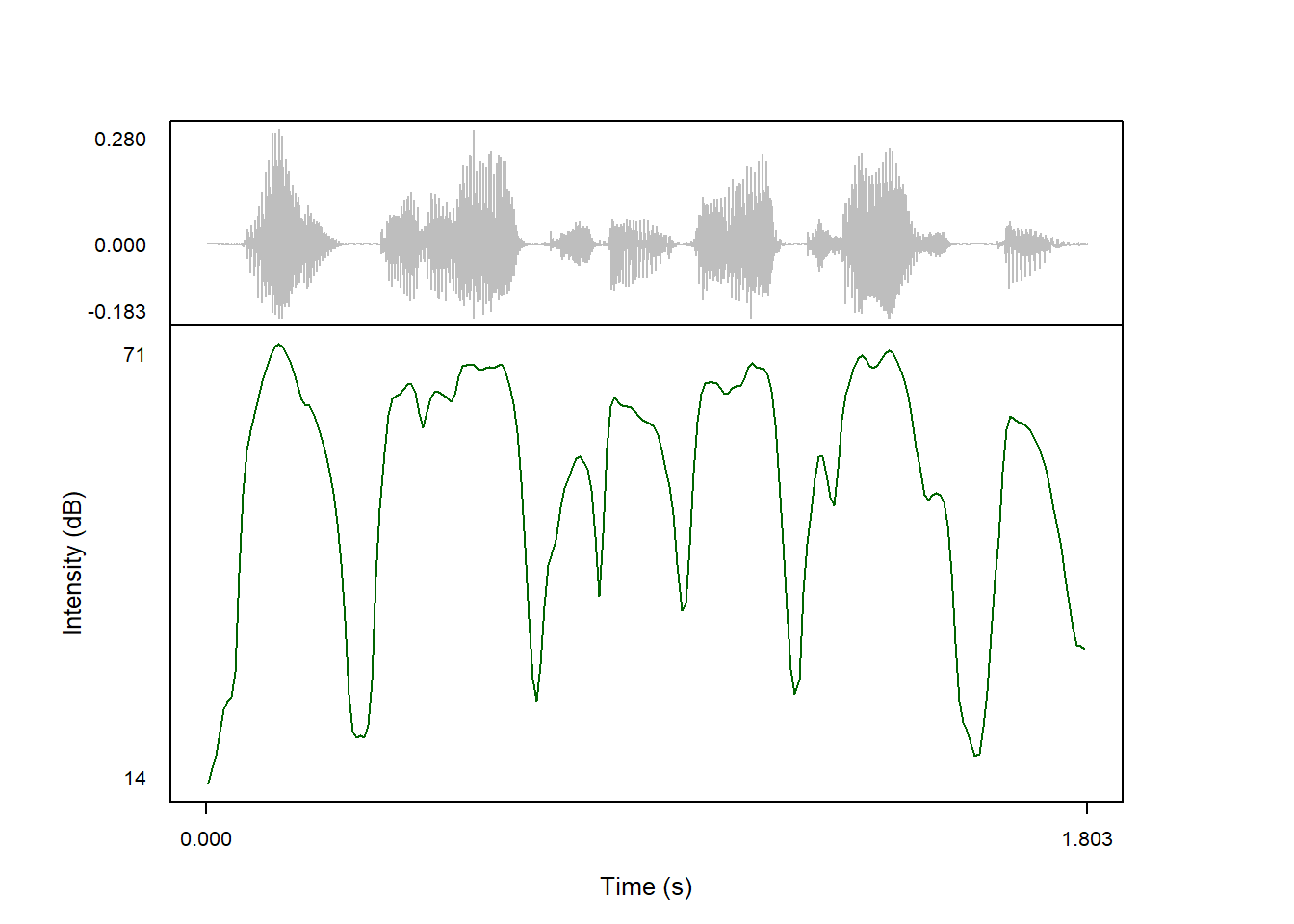
Some fancier coloring options are available when an intensity contour is overlaid on spectrograms; more on that in Section 8.1.5.
Users can specify their own axis labels, using the intensity_axisLabel argument. For example, we might want to use the term ‘root-mean-squared amplitude’, which is often used instead of ‘intensity’:
praatpicture('ex/ex.wav',
             frames = c('sound', 'intensity'),
             proportion = c(30,70),
             wave_color = 'grey',
             intensity_axisLabel = 'Root-mean-squared amplitude (dB)')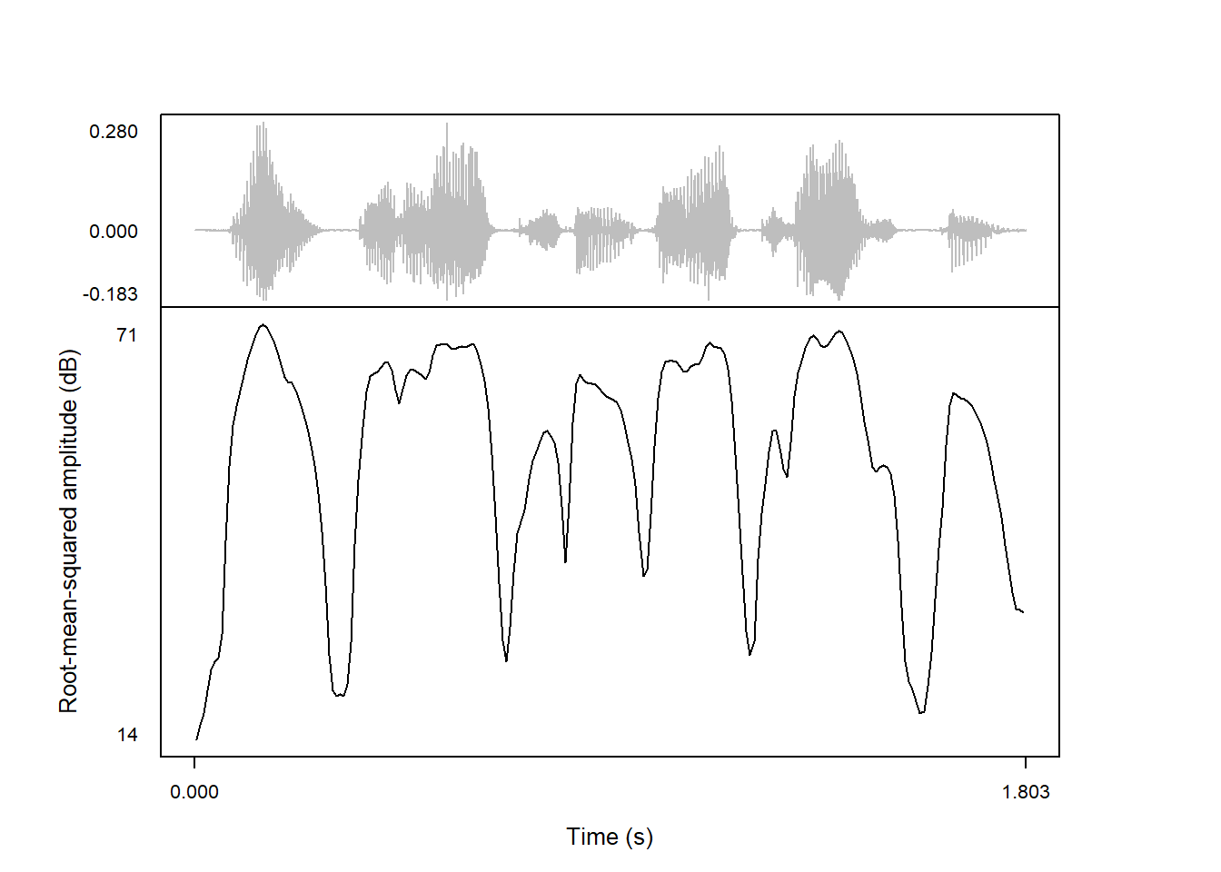
If you want to draw intensity contours with thicker, you can set the drawSize argument larger than 1 (which will also affect other drawn derived signals, i.e. pitch or formants).
praatpicture('ex/ex.wav',
             frames = c('sound', 'intensity'),
             proportion = c(30,70),
             wave_color = 'grey',
             drawSize = 3)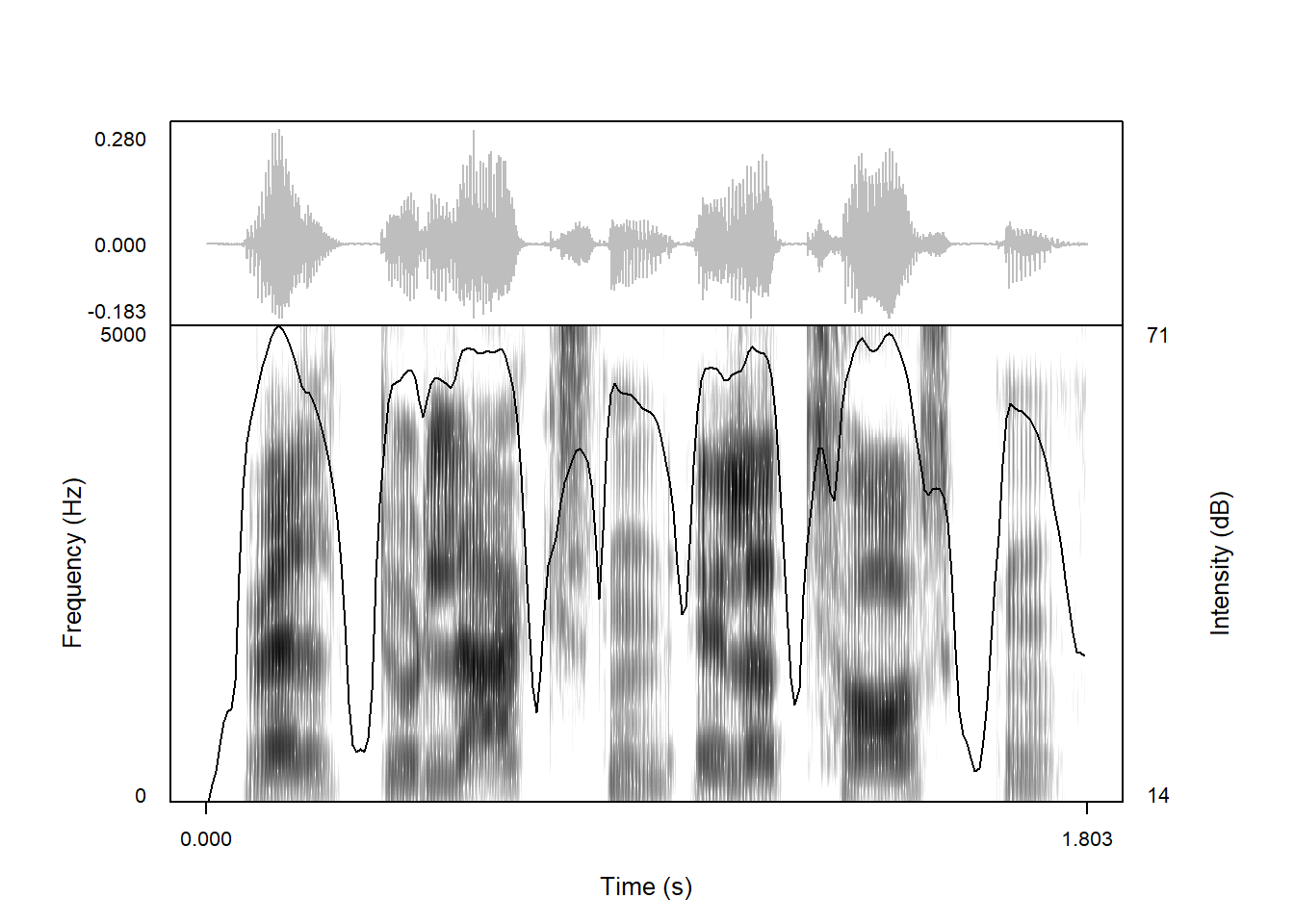
Instead of drawing intensity in its own frame, it is also possible to overlay an intensity contour on a spectrogram. In this case, intensity should not be specified as one of the frames; this is instead controlled with the Boolean intensity_plotOnSpec argument.
praatpicture('ex/ex.wav',
             frames = c('sound', 'spectrogram'),
             proportion = c(30,70),
             wave_color = 'grey',
             intensity_plotOnSpec = TRUE)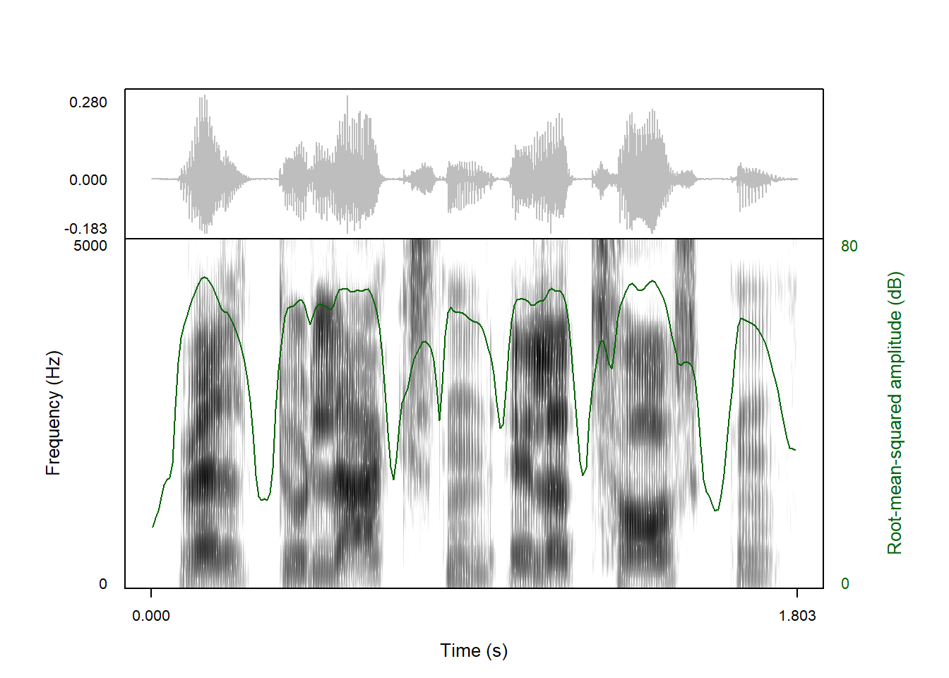
The other arguments controlling intensity appearance (and signal processing) also work when overlaying intensity on the spectrogram:
praatpicture('ex/ex.wav',
             frames = c('sound', 'spectrogram'),
             proportion = c(30,70),
             wave_color = 'grey',
             intensity_plotOnSpec = TRUE,
             intensity_range = c(0, 80),
             intensity_color = 'darkgreen',
             intensity_axisLabel = 'Root-mean-squared amplitude (dB)')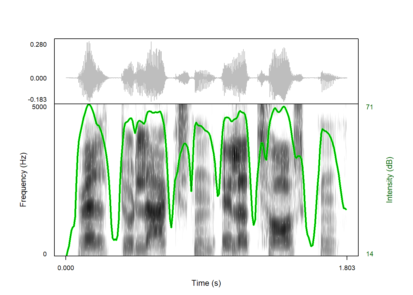
Notice that the y-axis label will match the color of the intensity contour.
When overlaying an intensity contour on a spectrogram, there is the added option of having a wider line with a separate background color, which helps the contour stand out more. For example, we may want the intensity contour in the above plot to have a lighter green background color. In this case, we can pass a vector to intensity_color specifying first the main color, and then the background:
praatpicture('ex/ex.wav',
             frames = c('sound', 'spectrogram'),
             proportion = c(30,70),
             wave_color = 'grey',
             intensity_plotOnSpec = TRUE,
             intensity_color = c('darkgreen', 'green'))
As you may have noticed, it’s possible to add either intensity, formants, or pitch traces on the spectrogram using the three separate arguments intensity_plotOnSpec, formant_plotOnSpec, and pitch_plotOnSpec. These do not cancel each other out; although it’s probably not recommended to do so – it makes for a very busy plot – you can choose to overlay all three on one spectrogram:
praatpicture('ex/ex.wav',
             frames = c('sound', 'spectrogram'),
             proportion = c(30,70),
             wave_color = 'grey',
             intensity_plotOnSpec = TRUE,
             intensity_color = c('darkgreen', 'green'),
             formant_plotOnSpec = TRUE,
             formant_color = c('red', 'pink'),
             pitch_plotOnSpec = TRUE,
             pitch_color = c('blue', 'lightblue'))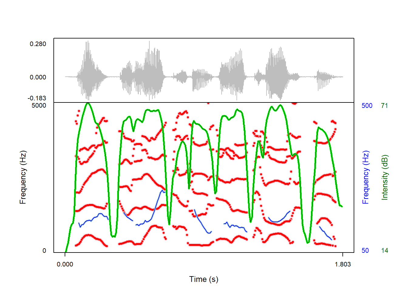
If you want multiple signals in one frame but don’t actually want the spectrogram, there’s a hack to do so: if you set the dynamic range of the spectrogram to 0 dB, it will simply be rendered as white, and if you then overlay other derived signals on the “spectrogram”, you will see just the other derived signals:
praatpicture('ex/ex.wav',
             frames = c('sound', 'spectrogram'),
             proportion = c(30,70),
             wave_color = 'grey',
             intensity_plotOnSpec = TRUE,
             intensity_color = c('darkgreen', 'green'),
             formant_plotOnSpec = TRUE,
             formant_color = c('red', 'pink'),
             pitch_plotOnSpec = TRUE,
             pitch_color = c('blue', 'lightblue'),
             spec_dynamicRange = 0)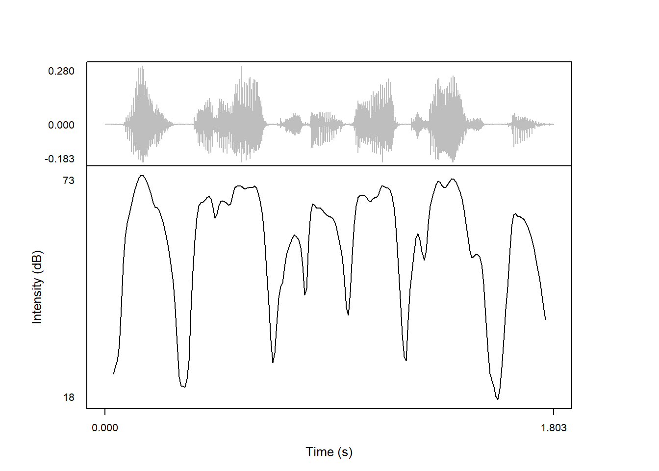
Intensity can also be overlaid on the waveform. This is controlled using the intensity_plotOnWave argument.
praatpicture('ex/ex.wav',
             frames = c('sound', 'spectrogram'),
             proportion = c(50,50),
             wave_color = 'grey',
             intensity_plotOnWave = TRUE)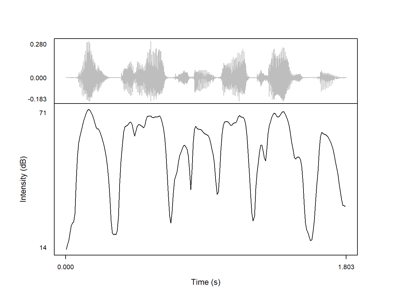
As with spectrogram overlays, all the other arguments controlling intensity appearance can still be controlled in the usual way:
praatpicture('ex/ex.wav',
             frames = c('sound', 'spectrogram'),
             proportion = c(50,50),
             wave_color = 'grey',
             intensity_plotOnWave = TRUE,
             intensity_range = c(0, 80),
             intensity_color = c('darkgreen','green'),
             intensity_axisLabel = 'Root-mean-squared amplitude (dB)')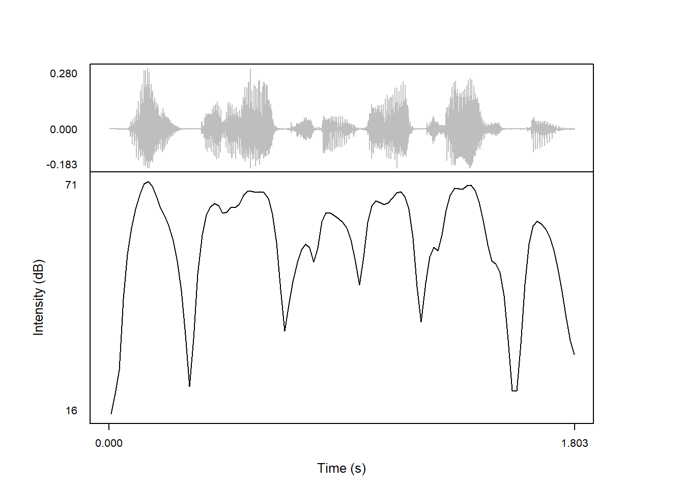
Intensity contours are typically calculated on the fly in R using the rmsana() function from the wrassp library, which is a convenient way to call functions from the C library libassp in R. rmsana() should in theory be implementing the same algorithm as Praat, but there will be some slight differences.
There are several reasons why you may wish to use the signal processing tools from Praat instead. If you’re writing about intensity and using Praat to generate the intensity contours, it could be important to show actual examples of the data you’re analyzing using the exact same parameter settings and the exact same algorithm as you’re using for the analysis. Luckily, it’s fairly straightforward to plot intensity contours in praatpicture that are calculated in Praat.
If you open and select a sound file in Praat, you can generate an intensity contour by clicking the To Intensity... button. Once you have done this, select the resulting Intensity object, and click the Down to IntensityTier button. Select this IntensityTier object, click the Save button, and select Save as text file..., and save the object using the same base name as your sound file and the .IntensityTier extension. If you have done this, praatpicture will automatically plot the values in the .IntensityTier file instead of calculating intensity on the fly.
As an example, this is a copy of the file that we’ve used throughout this section, which has a corresponding .IntensityTier file (i.e., intensity is calculated in Praat):
praatpicture('ex/ex_praatsp.wav',
             frames = c('sound', 'intensity'),
             proportion = c(30,70),
             wave_color = 'grey')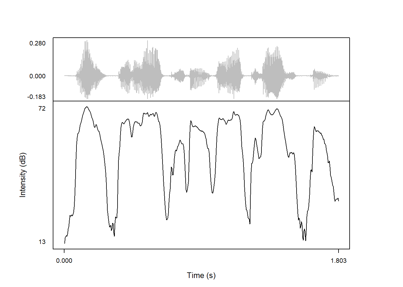
And this is that same snippet with intensity calculated in R on the fly:
praatpicture('ex/ex.wav',
             frames = c('sound', 'intensity'),
             proportion = c(30,70),
             wave_color = 'grey')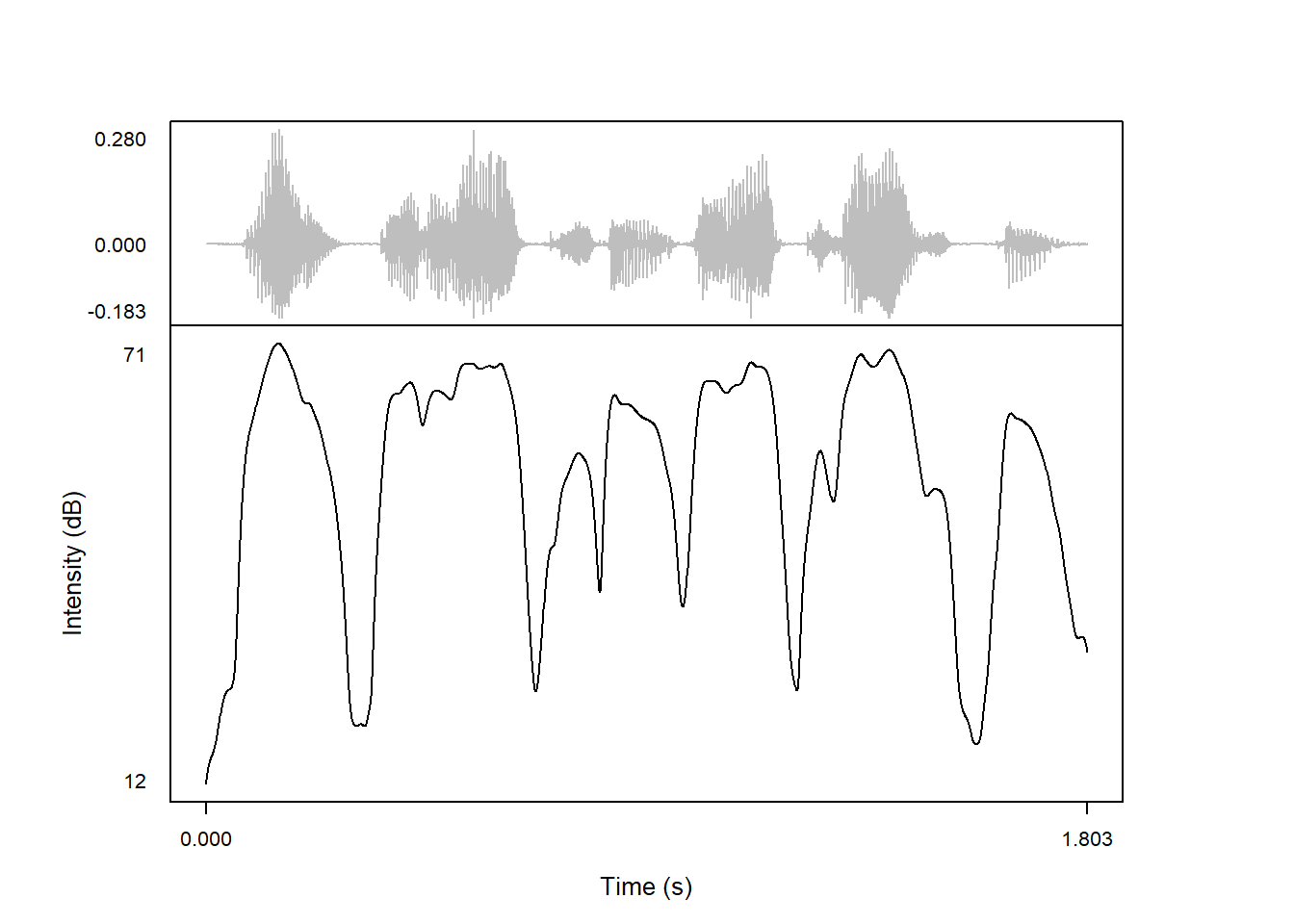
For most purposes, the intensity calculated on the fly in R will do just fine – there are only very slight differences in the resulting contour shapes.
Note that the signal processing options introduced below are only used when calculating intensity on the fly in R. If intensity is plotted from an .IntensityTier file, they are ignored – in this case, you need to set your own signal processing parameters in Praat!
The parameters used to predict pitch do not use rmsana() defaults, but are rather set to emulate Praat as closely as possible. Some of these can’t be changed (using Gaussian-shaped KAISER2_0 windows), but some can, in this case the same as those that can be toggled in Praat!
The default is to assume a minimum pitch of 100 Hz. That’s probably a bit high for this speaker, who does sometimes have pitch values below 100 Hz. With a minimum pitch of 50 Hz, we get smaller excursions:
praatpicture('ex/ex.wav',
             frames = c('sound', 'intensity'),
             proportion = c(30,70),
             wave_color = 'grey',
             intensity_minPitch = 50)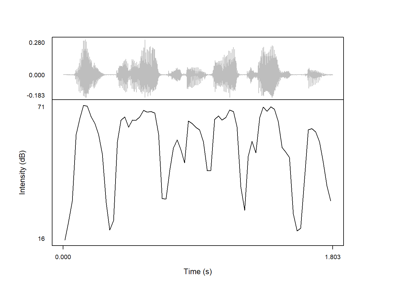
If we set minimum pitch too high, we get a very jagged contour:
praatpicture('ex/ex.wav',
             frames = c('sound', 'intensity'),
             proportion = c(30,70),
             wave_color = 'grey',
             intensity_minPitch = 200)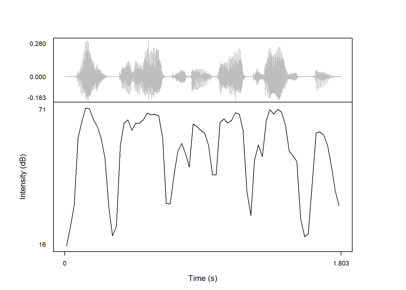
The intervals at which to measure intensity is controlled with the intensity_timeStep parameter. The default here is to calculate the measurement interval dynamically based on the intensity_minPitch, such that it is \(\frac{4}{5}\) / intensity_minPitch, which with the default minimum pitch of 100 Hz amounts to 0.008, i.e. every 80 ms. But users can also specify a number (in ms). Here we take a lot more measures, once per ms:
praatpicture('ex/ex.wav',
             frames = c('sound', 'intensity'),
             proportion = c(30,70),
             wave_color = 'grey',
             intensity_timeStep = 0.001)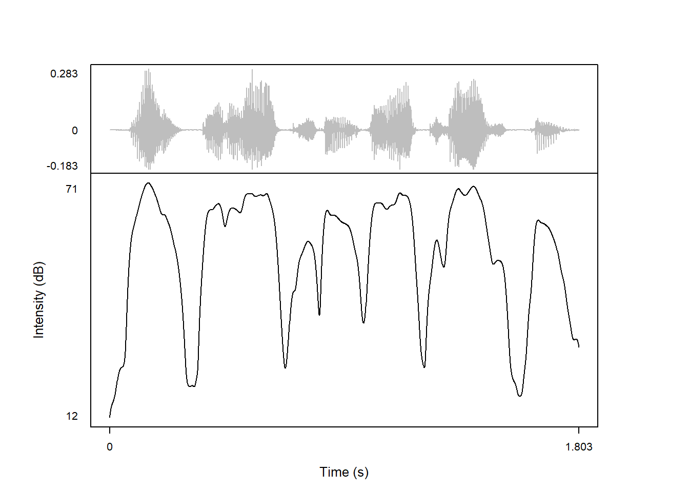
And this is what it looks like with fewer measures, once every 25 ms:
praatpicture('ex/ex.wav',
             frames = c('sound', 'intensity'),
             proportion = c(30,70),
             wave_color = 'grey',
             intensity_timeStep = 0.025)