praatpicture('ex/ex.wav')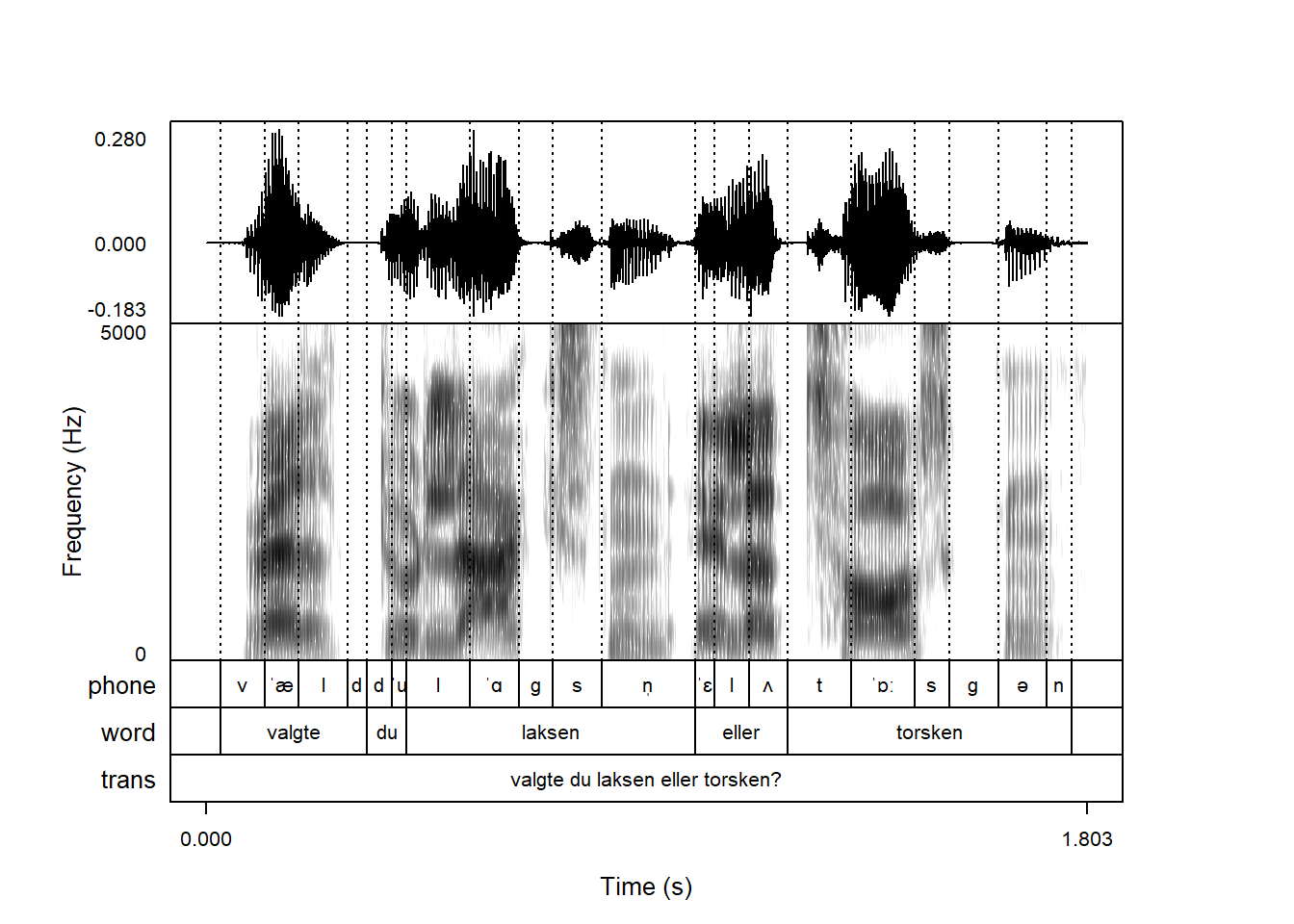
Let’s start with a very simple praatpicture call:
praatpicture('ex/ex.wav')
If you call praatpicture() with only a single argument giving the location of a sound file, as above, the function will look for the .wav file you passed, and also a .TextGrid file in the same directory with the same base name. You don’t have to plot annotations, but in that case you will have to tell praatpicture() using the frames argument as shown below. So if there’s no .TextGrid file, you will get an error. We will see later in Chapter 12 that it is also possible to annotate sound files interactively using R.
Very often you won’t want to plot an entire sound file. You can choose exactly which part of a sound file to plot with the start and end arguments, giving the start and end times of the plotted portion of the file in seconds:
praatpicture('ex/ex.wav',
             start = 1.2)
praatpicture('ex/ex.wav',
             end = 0.275)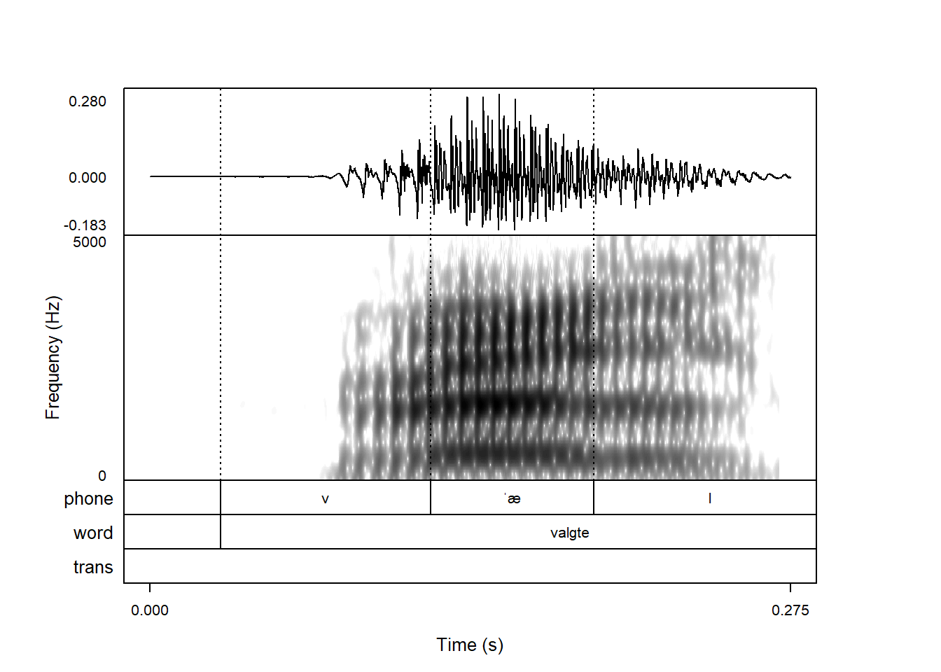
By default, praatpicture() plots a waveform, a spectrogram, and annotations. This is controlled with the frames argument, which takes any combination of the following options:
soundspectrogramTextGridpitchformantintensityThe default is to plot the first three, but we could also swap the spectrogram for formants:
praatpicture('ex/ex.wav',
             end = 0.275,
             frames = c('sound', 'formant', 'TextGrid'))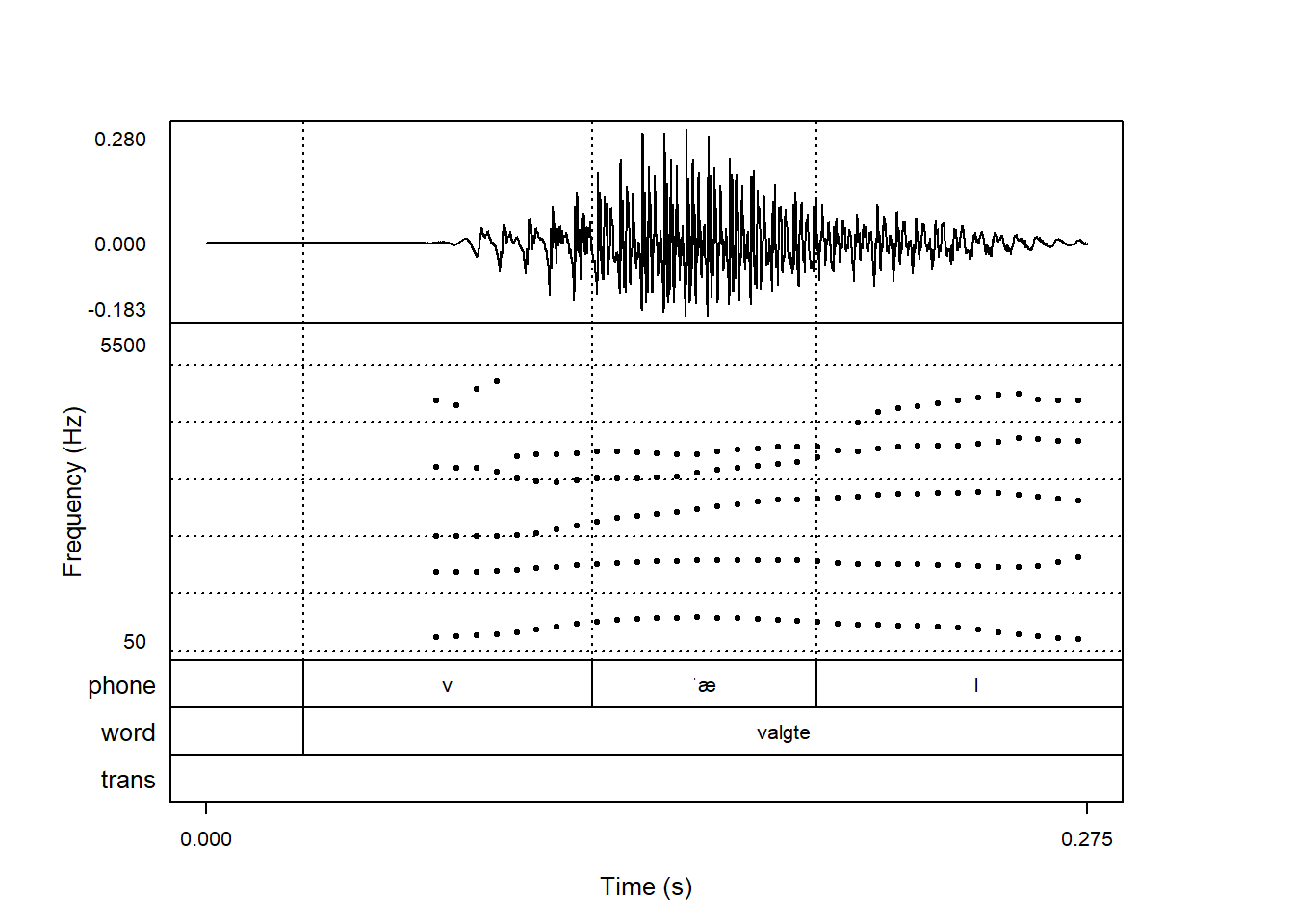
Or we could plot more frames:
praatpicture('ex/ex.wav',
             end = 0.275,
             frames = c('sound', 'spectrogram', 'intensity', 'TextGrid'))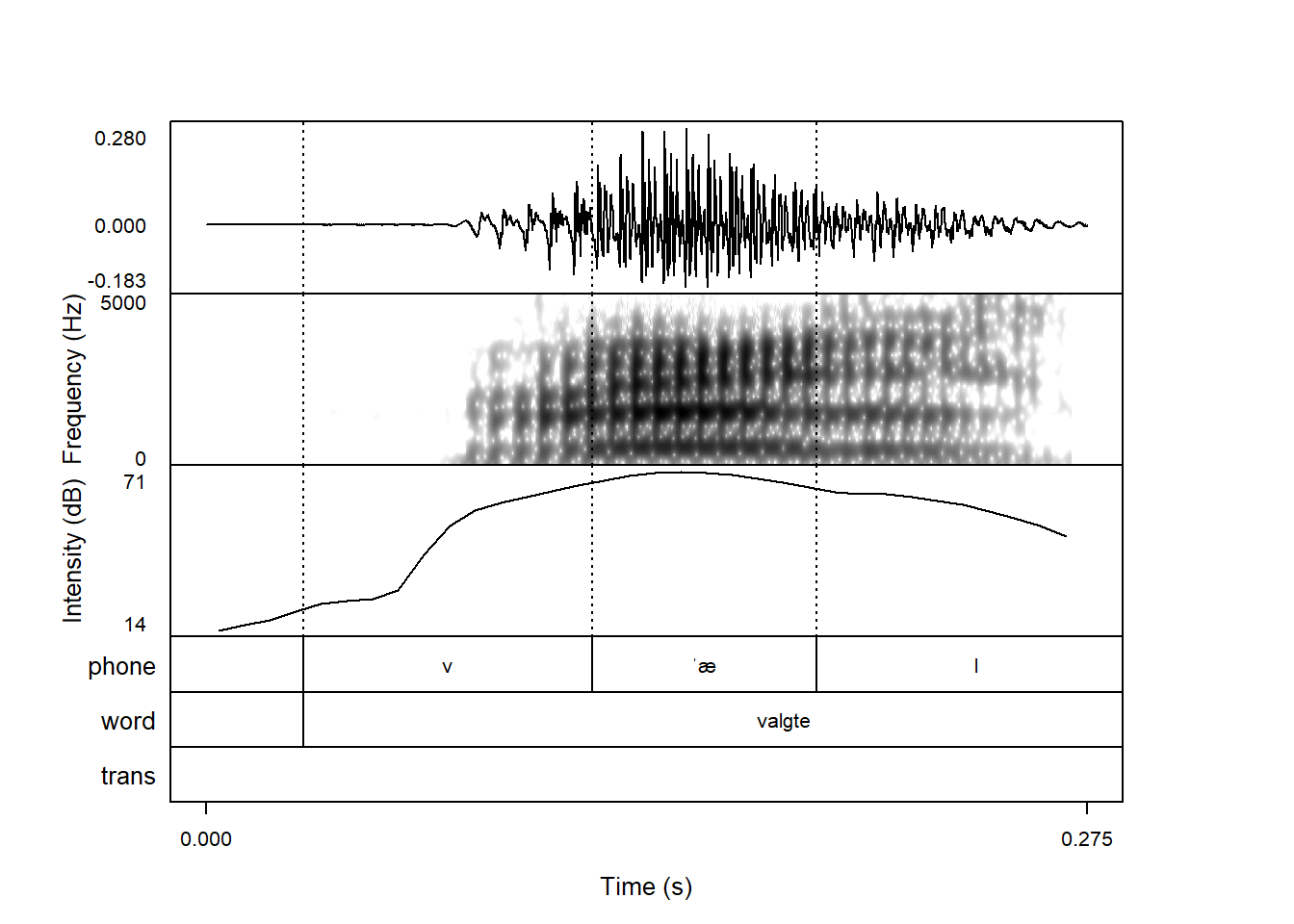
Or we could plot just a spectogram:
praatpicture('ex/ex.wav',
             end = 0.275,
             frames = 'spectrogram')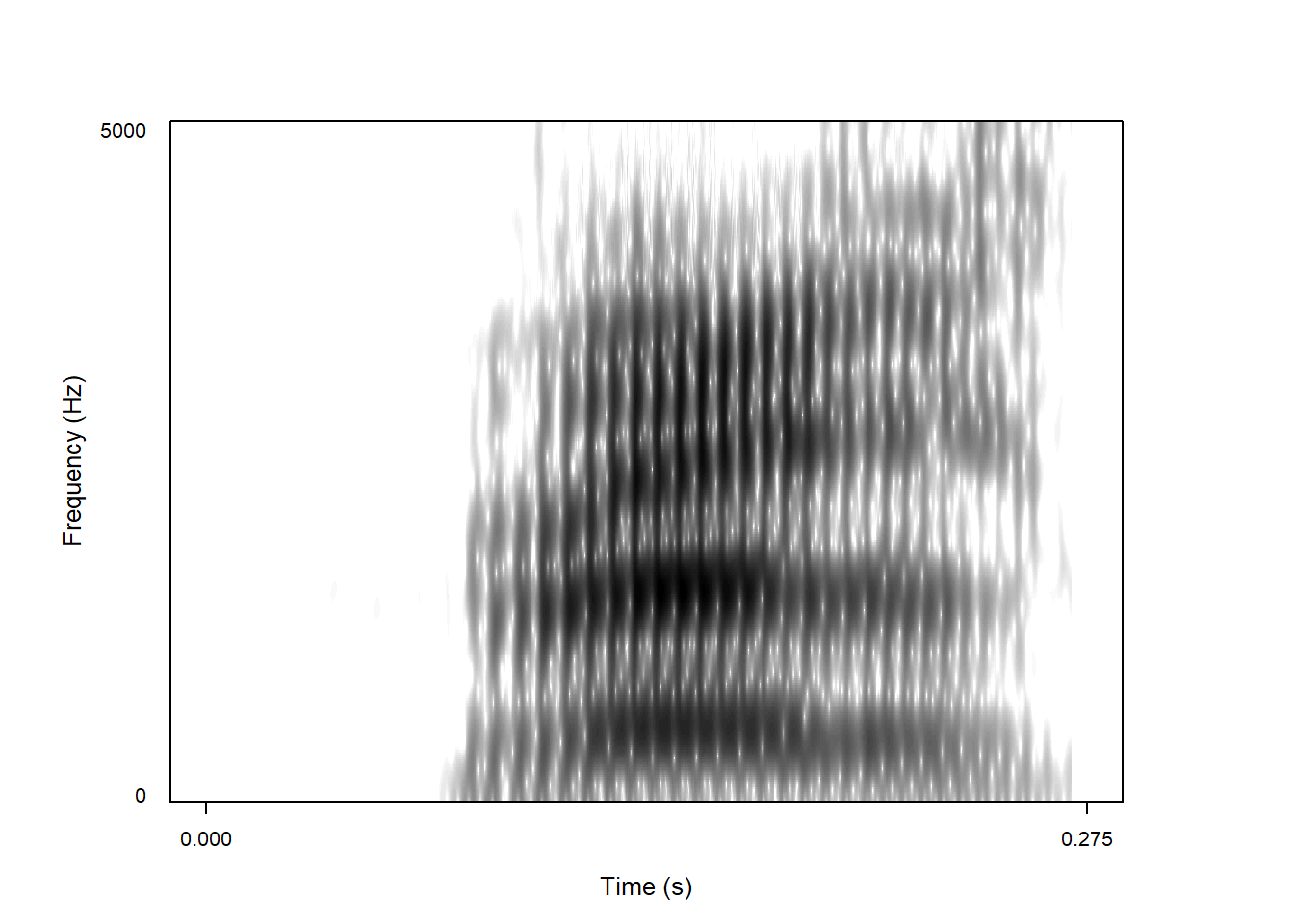
When using the default frames, the waveform is relatively small, the spectrogram is larger, and the annotations are smaller than either. When using more or less frames, they are all the same size. This can be controlled with the proportion argument, which gives the percentage in size of each component. The default is c(30,50,20), i.e. 30% waveform, 50% spectrogram, and 20% annotation.
The following reduces the size of the waveform and annotations to 15% each, and increases the size of the spectrogram to 70%:
praatpicture('ex/ex.wav',
             start = 1.2,
             proportion = c(15,70,15))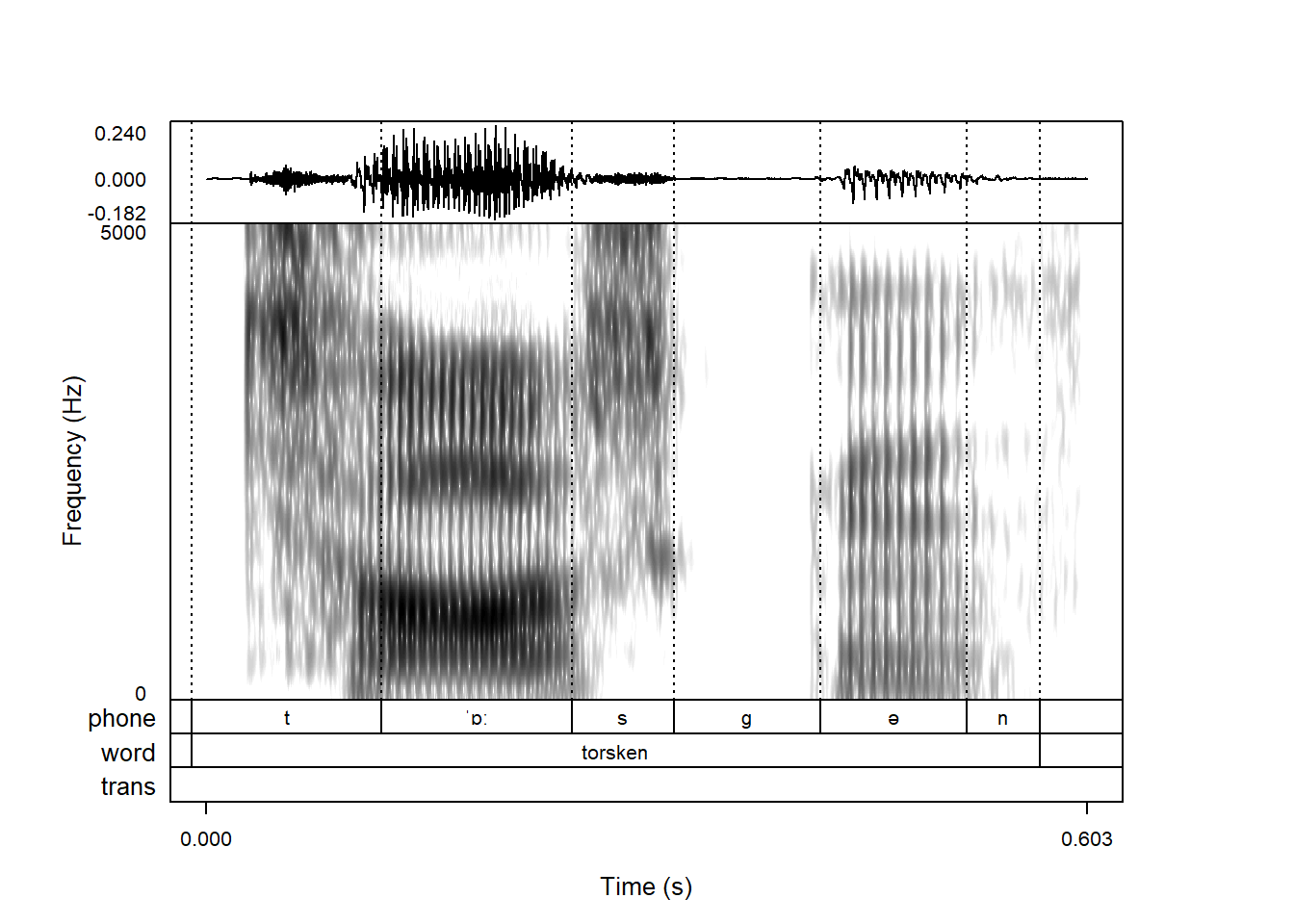
(It doesn’t really have to be percentages – passing c(3,5,2) for example would give the same result).
In accordance with Praat default settings, the default is to show only start and end times on the x-axis. This can be controlled with the start_end_only argument, which by default is set to TRUE:
praatpicture('ex/ex.wav',
             start = 1.2,
             start_end_only = FALSE)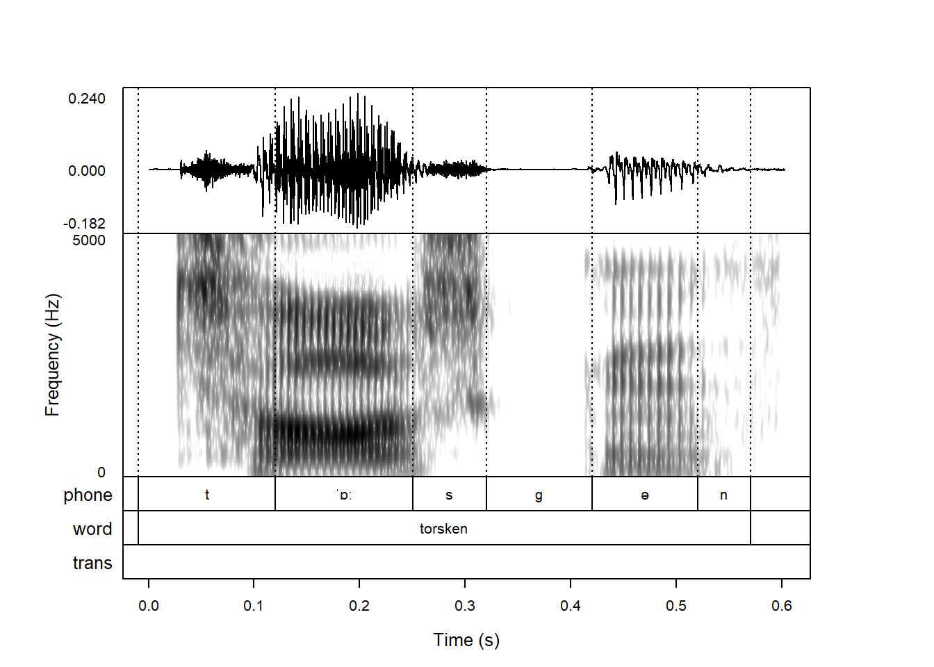
The x-axis starts at 0 by default even though in this case we actually start plotting 1.2 seconds into the sound file. This can be changed with the tfrom0 argument, which is also TRUE by default:
praatpicture('ex/ex.wav',
             start = 1.2,
             start_end_only = FALSE,
             tfrom0 = FALSE)
You can change the x-axis label using the time_axisLabel argument. If you prefer “Time in seconds” to “Time (s)”, this is easily done:
praatpicture('ex/ex.wav',
             start = 1.2,
             time_axisLabel = 'Time in seconds')
If you prefer your x-axis to be based on milliseconds rather than seconds, you can control this with the tUnit argument, which should then be set to tUnit = 'ms'.
praatpicture('ex/ex.wav',
             start = 1.2,
             tUnit = 'ms')
The y-axes, like the x-axes, also show only axis limits by default. This can be changed globally using the min_max_only argument, which is TRUE by default:
praatpicture('ex/ex.wav',
             start = 1.2,
             start_end_only = FALSE,
             min_max_only = FALSE)
As with the x-axis label, the y-axis labels can also all be controlled with specific arguments like pitch_axisLabel or other *_axisLabel arguments. We’ll cover this in the following sections.
All axes can be suppressed entirely using the suppressAxes argument. This is generally not recommended, but can come in handy for e.g. presentations.
praatpicture('ex/ex.wav',
             start = 1.2,
             suppressAxes = TRUE)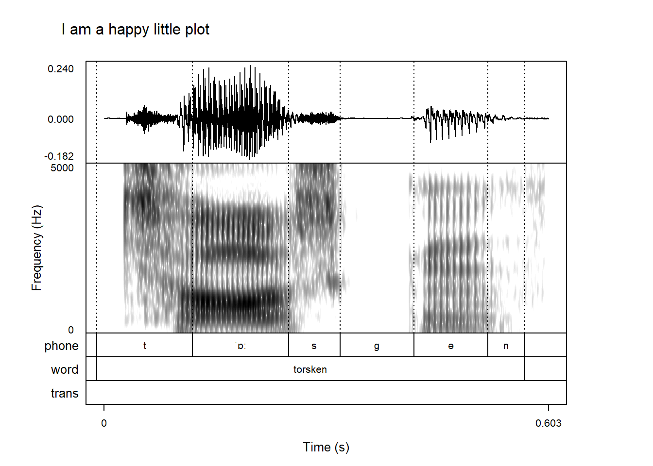
The argument mainTitle can be used to add a title on top of your plot, like this:
praatpicture('ex/ex.wav',
             start = 1.2,
             mainTitle = 'I am a happy little plot')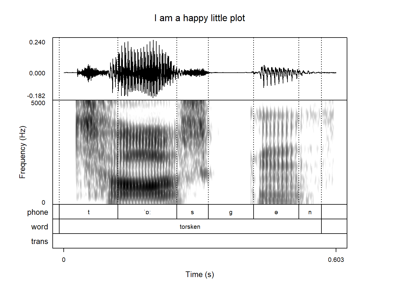
You can control the vertical aligment of the title with the mainTitleAlignment argument. This has to be a number between 0 and 1, where 0 is the left edge of the plot and 1 is the right edge of the plot. As such, 0.5 is a central title:
praatpicture('ex/ex.wav',
             start = 1.2,
             mainTitle = 'I am a happy little plot',
             mainTitleAlignment = 0.5)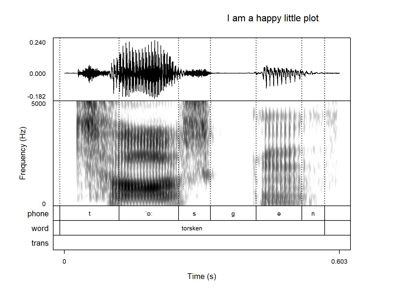
The title can be placed anywhere – this one is further to the right:
praatpicture('ex/ex.wav',
             start = 1.2,
             mainTitle = 'I am a happy little plot',
             mainTitleAlignment = 0.8)